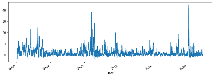
endog: The endogenous variable. the dependent variable (i.e. the target - 20 day max return)
k_regimes: The number of regimes.
trend: Whether or not to include a trend. Default is an intercept.
include an intercept: trend=’c’
include time trend: trend=’t’
include an intercept and time trend: trend=’ct’
no trend: trend=’n’
exog:exogenous regressors
switching_trend: whether or not all trend coefficients are switching across regimes. Default is True.
switching_exog:whether or not all regression coefficients are switching across regimes. Default is True.
switching_variance: Whether or not there is regime-specific heteroskedasticity, i.e. whether or not the error term has a switching variance. Default is False.
Summary
switching intercept: 2 regimes v. 5 regimes
set k_regimes as 2 or 5 and leave the rest as default
switching intercept and lagged dependent variable:
k_regimes = 3
lag 1 and lag20 as exog variables
importnumpyasnpimportpandasaspdimportstatsmodels.apiassmfromdatetimeimportdatetime,timedeltaimportyfinanceasyf#to download stock price data
#for each stock_id, get the max close in next 20 trading days
price_col='Close'roll_len=20new_col='next_20day_max'target_list=[]df.sort_index(ascending=True,inplace=True)df.head(3)
Markov switching with switching intercept: 2 regimes
set k_regimes=2: assuming 2 regimes
leave the rest as default
# Fit the model
# (a switching mean is the default of the MarkovRegession model)
markov_reg=sm.tsa.MarkovRegression(df['target'],k_regimes=2)res_target=markov_reg.fit()res_target.summary()
Markov Switching Model Results
Dep. Variable:
target
No. Observations:
5458
Model:
MarkovRegression
Log Likelihood
-13468.861
Date:
Sat, 06 Nov 2021
AIC
26947.723
Time:
21:37:15
BIC
26980.747
Sample:
0
HQIC
26959.246
- 5458
Covariance Type:
approx
Regime 0 parameters
coef
std err
z
P>|z|
[0.025
0.975]
const
1.6017
0.042
38.541
0.000
1.520
1.683
Regime 1 parameters
coef
std err
z
P>|z|
[0.025
0.975]
const
13.3001
0.237
56.154
0.000
12.836
13.764
Non-switching parameters
coef
std err
z
P>|z|
[0.025
0.975]
sigma2
7.5238
0.147
51.137
0.000
7.235
7.812
Regime transition parameters
coef
std err
z
P>|z|
[0.025
0.975]
p[0->0]
0.9946
0.001
923.936
0.000
0.992
0.997
p[1->0]
0.0701
0.014
5.182
0.000
0.044
0.097
Warnings: [1] Covariance matrix calculated using numerical (complex-step) differentiation.
note when P>
z
is not small (typically less than 0.05), we accept null hypothesis.
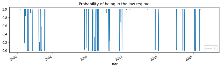
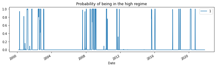
From the summary output, the first regime (the “low regime”) is estimated to be 1.6 whereas in the “high regime” it is 13.3. Below we plot the smoothed probabilities of being in the high regime.
res_target.smoothed_marginal_probabilities[[0]].plot(title="Probability of being in the low regime",figsize=(12,3))res_target.smoothed_marginal_probabilities[[1]].plot(title="Probability of being in the high regime",figsize=(12,3))
<AxesSubplot:title={'center':'Probability of being in the high regime'}, xlabel='Date'>
From the estimated transition matrix we can calculate the expected duration of a low regime versus a high regime.
print(res_target.expected_durations)
[185.00635239 14.26299654]
Markov switching with switching intercept: 5 regimes
set k_regimes=5: assuming 5 regimes
leave the rest as default
# Fit the model
# (a switching mean is the default of the MarkovRegession model)
markov_reg=sm.tsa.MarkovRegression(df['target'],k_regimes=5)res_target=markov_reg.fit()res_target.summary()
Markov Switching Model Results
Dep. Variable:
target
No. Observations:
5458
Model:
MarkovRegression
Log Likelihood
-10388.194
Date:
Sat, 06 Nov 2021
AIC
20828.388
Time:
21:39:57
BIC
21000.114
Sample:
0
HQIC
20888.309
- 5458
Covariance Type:
approx
Regime 0 parameters
coef
std err
z
P>|z|
[0.025
0.975]
const
0.5066
0.027
18.914
0.000
0.454
0.559
Regime 1 parameters
coef
std err
z
P>|z|
[0.025
0.975]
const
3.5746
0.072
49.828
0.000
3.434
3.715
Regime 2 parameters
coef
std err
z
P>|z|
[0.025
0.975]
const
7.7889
0.112
69.659
0.000
7.570
8.008
Regime 3 parameters
coef
std err
z
P>|z|
[0.025
0.975]
const
14.8677
0.140
106.019
0.000
14.593
15.143
Regime 4 parameters
coef
std err
z
P>|z|
[0.025
0.975]
const
30.9587
0.212
145.718
0.000
30.542
31.375
Non-switching parameters
coef
std err
z
P>|z|
[0.025
0.975]
sigma2
1.7108
0.036
47.337
0.000
1.640
1.782
Regime transition parameters
coef
std err
z
P>|z|
[0.025
0.975]
p[0->0]
0.9708
nan
nan
nan
nan
nan
p[1->0]
0.0780
0.001
55.775
0.000
0.075
0.081
p[2->0]
0.0213
nan
nan
nan
nan
nan
p[3->0]
0.0128
0.012
1.109
0.268
-0.010
0.035
p[4->0]
8.241e-06
0.000
0.019
0.985
-0.001
0.001
p[0->1]
0.0278
0.001
24.099
0.000
0.026
0.030
p[1->1]
0.8680
0.001
1313.738
0.000
0.867
0.869
p[2->1]
0.1157
0.005
24.987
0.000
0.107
0.125
p[3->1]
0.0137
0.012
1.183
0.237
-0.009
0.036
p[4->1]
3.511e-06
0.001
0.004
0.997
-0.002
0.002
p[0->2]
0.0013
0.002
0.563
0.574
-0.003
0.006
p[1->2]
0.0540
nan
nan
nan
nan
nan
p[2->2]
0.8007
0.027
30.029
0.000
0.748
0.853
p[3->2]
0.1635
6.57e-10
2.49e+08
0.000
0.164
0.164
p[4->2]
1.364e-06
0.000
0.003
0.998
-0.001
0.001
p[0->3]
1.016e-05
nan
nan
nan
nan
nan
p[1->3]
6.434e-05
0.002
0.028
0.978
-0.004
0.005
p[2->3]
0.0623
5.27e-07
1.18e+05
0.000
0.062
0.062
p[3->3]
0.8100
4.42e-09
1.83e+08
0.000
0.810
0.810
p[4->3]
8.906e-07
4.43e-07
2.009
0.045
2.16e-08
1.76e-06
Warnings: [1] Covariance matrix calculated using numerical (complex-step) differentiation.
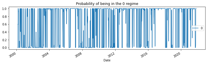
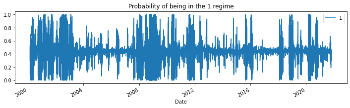
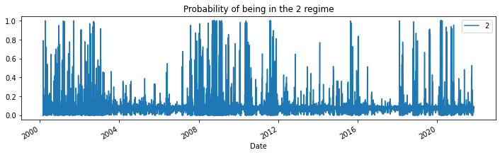
foriinrange(5):res_target.smoothed_marginal_probabilities[[i]].plot(title=f"Probability of being in the {i} regime",figsize=(12,3))
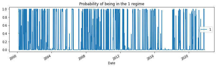
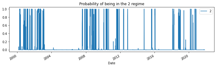
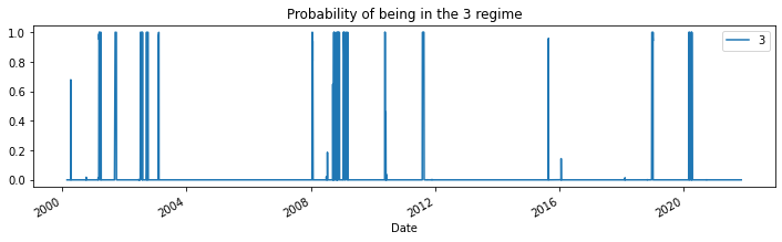
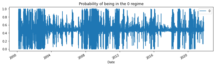
Markov switching with switching intercept and exogenous variables
set k_regimes=3: assuming 3 regimes
lag 1 and lag20 as exogenous variables
Because the models can be often difficult to estimate, for the 3-regime model we employ a search over starting parameters to improve results, specifying 50 random search repetitions.
# Fit the model
# (a switching mean is the default of the MarkovRegession model)
markov_reg=sm.tsa.MarkovRegression(df['target'],k_regimes=3,exog=df[['lag1','lag20']])res_target=markov_reg.fit()res_target.summary()
Markov Switching Model Results
Dep. Variable:
target
No. Observations:
5458
Model:
MarkovRegression
Log Likelihood
-8402.891
Date:
Sat, 06 Nov 2021
AIC
16837.782
Time:
21:40:27
BIC
16943.459
Sample:
0
HQIC
16874.656
- 5458
Covariance Type:
approx
Regime 0 parameters
coef
std err
z
P>|z|
[0.025
0.975]
const
0.2457
0.030
8.124
0.000
0.186
0.305
x1
0.7263
0.006
121.947
0.000
0.715
0.738
x2
-0.0624
0.006
-10.622
0.000
-0.074
-0.051
Regime 1 parameters
coef
std err
z
P>|z|
[0.025
0.975]
const
0.0278
0.034
0.821
0.412
-0.039
0.094
x1
0.9996
0.006
171.072
0.000
0.988
1.011
x2
0.0788
0.008
9.287
0.000
0.062
0.095
Regime 2 parameters
coef
std err
z
P>|z|
[0.025
0.975]
const
0.3858
0.118
3.274
0.001
0.155
0.617
x1
1.3538
0.014
98.518
0.000
1.327
1.381
x2
0.0428
0.016
2.653
0.008
0.011
0.074
Non-switching parameters
coef
std err
z
P>|z|
[0.025
0.975]
sigma2
0.8872
0.021
42.126
0.000
0.846
0.928
Regime transition parameters
coef
std err
z
P>|z|
[0.025
0.975]
p[0->0]
0.5232
0.039
13.336
0.000
0.446
0.600
p[1->0]
0.4120
0.029
14.022
0.000
0.354
0.470
p[2->0]
0.3652
0.055
6.611
0.000
0.257
0.473
p[0->1]
0.4031
0.041
9.779
0.000
0.322
0.484
p[1->1]
0.4723
0.034
14.089
0.000
0.407
0.538
p[2->1]
0.5848
0.057
10.222
0.000
0.473
0.697
Warnings: [1] Covariance matrix calculated using numerical (complex-step) differentiation.
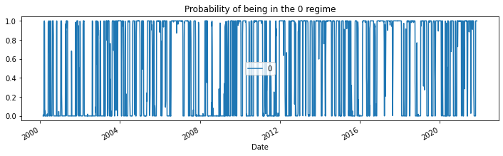
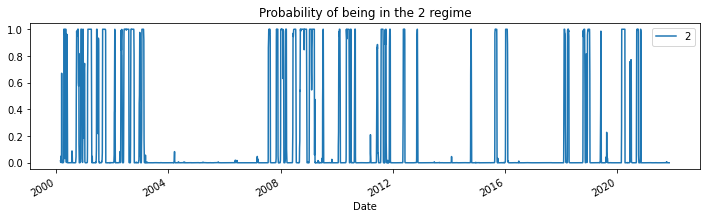
foriinrange(3):res_target.smoothed_marginal_probabilities[[i]].plot(title=f"Probability of being in the {i} regime",figsize=(12,3))