MAMA - MESA Adaptive Moving Average | Quantitative Research

MAMA: MESA Adaptive Moving Average

Reference:

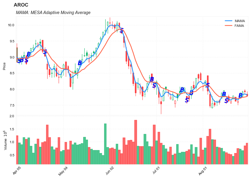
John Ehlers: MESA Adaptive Moving Average

MAMA: MESA Adaptive Moving Average

The MESA Adaptive Moving Average (MAMA) adapts to price movement based on the rate change of phase as measured by the Hilbert Transform Discriminator.

The advantage of this method of adaptation is that it features a fast attack average and a slow decay average so that composite average rapidly ratchets behind price changes and holds the average value until the next ratchet occurs.

Load basic packages

import pandas as pd
import numpy as np
import os
import gc
import copy
from pathlib import Path
from datetime import datetime, timedelta, time, date

#this package is to download equity price data from yahoo finance
#the source code of this package can be found here: https://github.com/ranaroussi/yfinance/blob/main
import yfinance as yf

pd.options.display.max_rows = 100
pd.options.display.max_columns = 100

import warnings
warnings.filterwarnings("ignore")

import pytorch_lightning as pl
random_seed=1234
pl.seed_everything(random_seed)

Global seed set to 1234

1234

#S&P 500 (^GSPC),  Dow Jones Industrial Average (^DJI), NASDAQ Composite (^IXIC)
#Russell 2000 (^RUT), Crude Oil Nov 21 (CL=F), Gold Dec 21 (GC=F)
#Treasury Yield 10 Years (^TNX)

#benchmark_tickers = ['^GSPC', '^DJI', '^IXIC', '^RUT',  'CL=F', 'GC=F', '^TNX']

benchmark_tickers = ['^GSPC']
tickers = benchmark_tickers + ['GSK', 'NVO', 'AROC']

#https://github.com/ranaroussi/yfinance/blob/main/yfinance/base.py
#     def history(self, period="1mo", interval="1d",
#                 start=None, end=None, prepost=False, actions=True,
#                 auto_adjust=True, back_adjust=False,
#                 proxy=None, rounding=False, tz=None, timeout=None, **kwargs):

dfs = {}

for ticker in tickers:
    cur_data = yf.Ticker(ticker)
    hist = cur_data.history(period="max", start='2000-01-01')
    print(datetime.now(), ticker, hist.shape, hist.index.min(), hist.index.max())
    dfs[ticker] = hist

2022-08-27 13:58:24.342430 ^GSPC (5701, 7) 1999-12-31 00:00:00 2022-08-26 00:00:00
2022-08-27 13:58:24.638344 GSK (5701, 7) 1999-12-31 00:00:00 2022-08-26 00:00:00
2022-08-27 13:58:24.982461 NVO (5701, 7) 1999-12-31 00:00:00 2022-08-26 00:00:00
2022-08-27 13:58:25.208361 AROC (3782, 7) 2007-08-21 00:00:00 2022-08-26 00:00:00

ticker = 'AROC'
dfs[ticker].tail(5)

	Open	High	Low	Close	Volume	Dividends	Stock Splits
Date
2022-08-22	7.59	7.68	7.50	7.62	753700	0.0	0
2022-08-23	7.74	7.90	7.71	7.80	732200	0.0	0
2022-08-24	7.78	7.95	7.74	7.92	673800	0.0	0
2022-08-25	7.95	8.00	7.84	7.92	857000	0.0	0
2022-08-26	7.85	7.93	7.76	7.79	962900	0.0	0

Define MAMA calculation function

def cal_mama(ohlc: pd.DataFrame, fast_limit: float = 0.5, slow_limit: float = 0.05, column: str = "close",) -> pd.DataFrame:
    """
    MESA Adaptive Moving Average

    The MESA Adaptive Moving Average (MAMA) adapts to price movement based on the rate change of phase as 
    measured by the Hilbert Transform Discriminator.  

    The advantage of this method of adaptation is that it features a fast attack average and a slow decay 
    average so that composite average rapidly ratchets behind price changes and holds the average value 
    until the next ratchet occurs.


    source: https://www.mesasoftware.com/papers/MAMA.pdf

    adapted from: https://github.com/mathiswellmann/go_ehlers_indicators/blob/bdc7bd10003c/mama.go#L110


    """
    series = ohlc[column]
    smooth = np.zeros(len(series))
    period = np.zeros(len(series))
    detrender = np.zeros(len(series))
    i1 = np.zeros(len(series))
    q1 = np.zeros(len(series))
    ji = np.zeros(len(series))
    jq = np.zeros(len(series))
    i2 = np.zeros(len(series))
    q2 = np.zeros(len(series))
    re = np.zeros(len(series))
    im = np.zeros(len(series))

    smooth_period = np.zeros(len(series))
    phase = np.zeros(len(series))
    fama = np.zeros(len(series))
    mama = np.zeros(len(series))

    delta_phase = np.zeros(len(series))    
    alpha = np.zeros(len(series))

    vals = series.values

    for i in range(len(vals)):
        if i<6:
            mama[i] = vals[i]
            fama[i] = vals[i]
            continue

        smooth[i] = (4*vals[i] + 3*vals[i-1] + 2*vals[i-2] + vals[i-3]) / 10
        detrender[i] = (0.0962*smooth[i] + 0.5769*smooth[i-2] - 0.5769*smooth[i-4] - 0.0962*smooth[i-6]) * (0.075*period[i-1] + 0.54)

        ## compute InPhase and Quadrature components
        q1[i] = (0.0962*detrender[i] + 0.5769*detrender[i-2] - 0.5769*detrender[i-4] - 0.0962*detrender[i-6]) * (0.075*period[i-1] + 0.54)
        i1[i] = detrender[i-3]


        ##Advance the phase of detrender and q1 by 90 Degrees
        ji[i] = (0.0962*i1[i] + 0.05769*i1[i-2] - 0.5769*i1[i-4] - 0.0962*i1[i-6]) * (0.075*period[i-1] + 0.54)
        jq[i] = (0.0962*q1[i] + 0.5769*q1[i-2] - 0.5769*q1[i-4] - 0.0962*q1[i-6]) * (0.075*period[i-1] + 0.54)

        ##Phasor addition for 3 bar averaging
        i2[i] = i1[i] - jq[i]
        q2[i] = q1[i] + ji[i]

        ##smooth the I and Q components befor applying the discriminator
        i2[i] = 0.2*i2[i] + 0.8*i2[i-1]
        q2[i] = 0.2*q2[i] + 0.8*q2[i-1]

        ##Homodyne Discriminator
        re[i] = i2[i]*i2[i-1] + q2[i]*q2[i-1]
        im[i] = i2[i]*q2[i-1] - q2[i]*i2[i-1]

        re[i] = 0.2*re[i] + 0.8*re[i-1]
        im[i] = 0.2*im[i] + 0.8*im[i-1]

        if (im[i] != 0)& (re[i] != 0):
            period[i] = 360 / np.arctan(im[i]/re[i])

        if (period[i] > 1.5*period[i-1]):
            period[i] = 1.5 * period[i-1]

        if (period[i] < 0.67*period[i-1]):
            period[i] = 0.67 * period[i-1]

        if (period[i] < 6):
            period[i] = 6

        if (period[i] > 50):
            period[i] = 50

        period[i] = 0.2*period[i] + 0.8*period[i-1]
        smooth_period[i] = 0.33*period[i] + 0.67*smooth_period[i-1]

        if (i1[i]!= 0):
            phase[i] = np.arctan(q1[i] / i1[i])

        delta_phase[i] = phase[i-1] - phase[i]
        if (delta_phase[i] < 1):
            delta_phase[i] = 1

        alpha[i] = fast_limit / delta_phase[i]
        if alpha[i] < slow_limit:
            alpha[i] = slow_limit

        mama[i] = alpha[i]*vals[i] + (1-alpha[i])*mama[i-1]
        fama[i] = 0.5*alpha[i]*mama[i] + (1-0.5*alpha[i])*fama[i-1]

    mama_ = pd.Series(index=series.index, data=mama, name="MAMA")
    fama_ = pd.Series(index=series.index, data=fama, name="FAMA")


    return pd.concat([mama_, fama_], axis=1)

def get_MAMA_signal(df):
    signals = []
    df.sort_index(ascending=True, inplace=True)
    M_F = df['MAMA']-df['FAMA']
    MAMA = df['MAMA']  
    
    for i in range(df.shape[0]):
        val = 0 #not a crossing point
        
        if M_F[i]==0:
            if i<2:
                val = 0
            else:
                if (M_F[i-1]<0):
                    val = 1 #from MAMA<FAMA to MAMA>FAMA
                elif (M_F[i-1]>0):
                    val = -1 #from MAMA>FAMA to MAMA<FAMA
                else:
                    val = 0
        else:
            if (i<2)|(i>=df.shape[0]-2):
                val = 0
            else:
                if (M_F[i-1]<0) & (M_F[i]>0):
                    val = 2
                elif (M_F[i-1]>0) & (M_F[i]<0):
                    val = -2
                else:
                    val = 0

        signals.append(val)
        
    return signals

Calculate MAMA

df = dfs[ticker][['Open', 'High', 'Low', 'Close', 'Volume']]

df = df.round(2)

help(cal_mama)

Help on function cal_mama in module __main__:

cal_mama(ohlc: pandas.core.frame.DataFrame, fast_limit: float = 0.5, slow_limit: float = 0.05, column: str = 'close') -> pandas.core.frame.DataFrame
    MESA Adaptive Moving Average
    
    The MESA Adaptive Moving Average (MAMA) adapts to price movement based on the rate change of phase as 
    measured by the Hilbert Transform Discriminator.  
    
    The advantage of this method of adaptation is that it features a fast attack average and a slow decay 
    average so that composite average rapidly ratchets behind price changes and holds the average value 
    until the next ratchet occurs.
    
    
    source: https://www.mesasoftware.com/papers/MAMA.pdf
    
    adapted from: https://github.com/mathiswellmann/go_ehlers_indicators/blob/bdc7bd10003c/mama.go#L110

df_ta = cal_mama(df, column="Close")
df = df.merge(df_ta, left_index = True, right_index = True, how='inner' )

del df_ta
gc.collect()

signals = get_MAMA_signal(df)
df['MAMA_signal'] = signals
df['B'] = (df["MAMA_signal"]>0) .astype(int)*(df['High']+df['Low'])/2
df['S'] = (df["MAMA_signal"]<0).astype(int)*(df['High']+df['Low'])/2

display(df.head(5))
display(df.tail(5))

	Open	High	Low	Close	Volume	MAMA	FAMA	MAMA_signal	B	S
Date
2007-08-21	50.01	50.86	49.13	49.44	1029100	49.44	49.44	0	0.0	0.0
2007-08-22	48.50	50.70	47.78	49.29	996500	49.29	49.29	0	0.0	0.0
2007-08-23	49.76	49.82	47.56	48.03	742700	48.03	48.03	0	0.0	0.0
2007-08-24	47.93	48.77	47.87	48.58	416000	48.58	48.58	0	0.0	0.0
2007-08-27	48.56	48.81	46.85	47.47	447000	47.47	47.47	0	0.0	0.0

	Open	High	Low	Close	Volume	MAMA	FAMA	MAMA_signal	B	S
Date
2022-08-22	7.59	7.68	7.50	7.62	753700	7.659967	7.706288	0	0.000	0.0
2022-08-23	7.74	7.90	7.71	7.80	732200	7.729984	7.712212	2	7.805	0.0
2022-08-24	7.78	7.95	7.74	7.92	673800	7.824992	7.740407	0	0.000	0.0
2022-08-25	7.95	8.00	7.84	7.92	857000	7.846852	7.752653	0	0.000	0.0
2022-08-26	7.85	7.93	7.76	7.79	962900	7.818426	7.769096	0	0.000	0.0

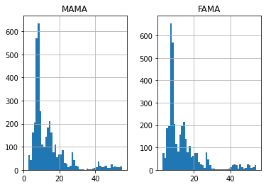
df[['MAMA','FAMA']].hist(bins=50)

array([[<AxesSubplot:title={'center':'MAMA'}>,
        <AxesSubplot:title={'center':'FAMA'}>]], dtype=object)

png

#https://github.com/matplotlib/mplfinance
#this package help visualize financial data
import mplfinance as mpf
import matplotlib.colors as mcolors

# all_colors = list(mcolors.CSS4_COLORS.keys())#"CSS Colors"
all_colors = list(mcolors.TABLEAU_COLORS.keys()) # "Tableau Palette",
# all_colors = list(mcolors.BASE_COLORS.keys()) #"Base Colors",


#https://github.com/matplotlib/mplfinance/issues/181#issuecomment-667252575
#list of colors: https://matplotlib.org/stable/gallery/color/named_colors.html
#https://github.com/matplotlib/mplfinance/blob/master/examples/styles.ipynb

def plot_3panels(main_data, add_data=None, mid_panel=None, chart_type='candle', names=None, 
                  figratio=(14,9)):


    style = mpf.make_mpf_style(base_mpf_style='yahoo',  #charles
                               base_mpl_style = 'seaborn-whitegrid',
#                                marketcolors=mpf.make_marketcolors(up="r", down="#0000CC",inherit=True),
                               gridcolor="whitesmoke", 
                               gridstyle="--", #or None, or - for solid
                               gridaxis="both", 
                               edgecolor = 'whitesmoke',
                               facecolor = 'white', #background color within the graph edge
                               figcolor = 'white', #background color outside of the graph edge
                               y_on_right = False,
                               rc =  {'legend.fontsize': 'small',#or number
                                      #'figure.figsize': (14, 9),
                                     'axes.labelsize': 'small',
                                     'axes.titlesize':'small',
                                     'xtick.labelsize':'small',#'x-small', 'small','medium','large'
                                     'ytick.labelsize':'small'
                                     }, 
                              )   

    if (chart_type is None) or (chart_type not in ['ohlc', 'line', 'candle', 'hollow_and_filled']):
        chart_type = 'candle'
    len_dict = {'candle':2, 'ohlc':3, 'line':1, 'hollow_and_filled':2}    
        
    kwargs = dict(type=chart_type, figratio=figratio, volume=True, volume_panel=1, 
                  panel_ratios=(4,2), tight_layout=True, style=style, returnfig=True)
    
    if names is None:
        names = {'main_title': '', 'sub_tile': ''}
    


    added_plots = { 
        'S':  mpf.make_addplot(add_data['S'], panel=0, color='blue', type='scatter', marker=r'${S}$' , markersize=100, secondary_y=False),   
        'B':  mpf.make_addplot(add_data['B'], panel=0, color='blue', type='scatter', marker=r'${B}$' , markersize=100, secondary_y=False), 
        
        'MAMA': mpf.make_addplot(add_data['MAMA'], panel=0, color='dodgerblue', secondary_y=False), 
        'FAMA': mpf.make_addplot(add_data['FAMA'], panel=0, color='tomato', secondary_y=False), 
#         'AO-SIGNAL': mpf.make_addplot(mid_panel['AO']-mid_panel['SIGNAL'], type='bar',width=0.7,panel=1, color="pink",alpha=0.65,secondary_y=False),
    }

                         

    fig, axes = mpf.plot(main_data,  **kwargs,
                         addplot=list(added_plots.values()),
                        )
    # add a new suptitle
    fig.suptitle(names['main_title'], y=1.05, fontsize=12, x=0.128)

    axes[0].set_title(names['sub_tile'], fontsize=10, style='italic',  loc='left')
    
    

    
    #set legend

    axes[0].legend([None]*6)
    handles = axes[0].get_legend().legendHandles
#     print(handles)
    axes[0].legend(handles=handles[4:],labels=['MAMA', 'FAMA'])
    #axes[2].set_title('AO', fontsize=10, style='italic',  loc='left')
#     axes[0].set_ylabel('MAMA')
    
    

#     axes[0].set_ylabel(names['y_tiles'][0])
    return fig, axes
   

start = -100
end = df.shape[0]

names = {'main_title': f'{ticker}', 
         'sub_tile': 'MAMA: MESA Adaptive Moving Average'}


aa_, bb_ = plot_3panels(df.iloc[start:end][['Open', 'High', 'Low', 'Close', 'Volume']], 
             df.iloc[start:end][['B', 'S', 'MAMA', 'FAMA']],
             None, 
             chart_type='hollow_and_filled',
                     names = names, 
                    )

png