Coppock Curve
References
Definition
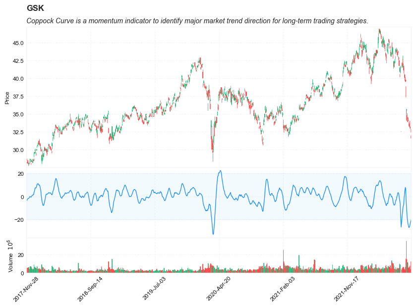
The Coppock Curve is a price momentum indicator to determine major lows in the stock market and is calculated as a moving average. The Coppock Curve is said to have been developed for long-term strategies involving indexes, ETFs, and other liquid instruments rather than intraday trading. The indicator can be used to identify major market trends, determine trend direction, and guide long-term investing or trading strategies.
The formula used for the Coppock Curve was developed in 1962 by Edwin S. Coppock in that year’s edition of Barron’s. The indicator was originally introduced as a long-term buy or sell indicator for major indices. It was first implemented this way to allow for indices to identify and target large trends.
Read the indicator
The Coppock Curve is an oscillating trendline that ranges both higher and lower than zero, incorporating two rates of change in its calculations:
11-period change; 14-period change.
The curve reviews the rate of change for these periods and then derives a signal line indicator that is extrapolated from this data, by using a 10-month weighted moving average. When using the curve, traders, investors, and technical analysts can look to the signal line indicator to help analyze and come to their own investment conclusions based on their findings for medium/long-term trades.
The Coppock Curve was created by an economist for medium to long-term trend analysis in indexes, ETFs, and other liquid instruments. It measures the rate of change and looks to present a clear trend for the medium and long-term.
Load basic packages
import pandas as pd
import numpy as np
import os
import gc
import copy
from pathlib import Path
from datetime import datetime, timedelta, time, date
#this package is to download equity price data from yahoo finance
#the source code of this package can be found here: https://github.com/ranaroussi/yfinance/blob/main
import yfinance as yf
pd.options.display.max_rows = 100
pd.options.display.max_columns = 100

import warnings
warnings.filterwarnings("ignore")

import pytorch_lightning as pl
random_seed=1234
pl.seed_everything(random_seed)
Global seed set to 1234


1234
#S&P 500 (^GSPC),  Dow Jones Industrial Average (^DJI), NASDAQ Composite (^IXIC)
#Russell 2000 (^RUT), Crude Oil Nov 21 (CL=F), Gold Dec 21 (GC=F)
#Treasury Yield 10 Years (^TNX)

#benchmark_tickers = ['^GSPC', '^DJI', '^IXIC', '^RUT',  'CL=F', 'GC=F', '^TNX']

benchmark_tickers = ['^GSPC']
tickers = benchmark_tickers + ['GSK', 'NVO', 'PFE', 'DAL']
#https://github.com/ranaroussi/yfinance/blob/main/yfinance/base.py
#     def history(self, period="1mo", interval="1d",
#                 start=None, end=None, prepost=False, actions=True,
#                 auto_adjust=True, back_adjust=False,
#                 proxy=None, rounding=False, tz=None, timeout=None, **kwargs):

dfs = {}

for ticker in tickers:
    cur_data = yf.Ticker(ticker)
    hist = cur_data.history(period="max", start='2000-01-01')
    print(datetime.now(), ticker, hist.shape, hist.index.min(), hist.index.max())
    dfs[ticker] = hist
2022-09-05 18:12:13.916297 ^GSPC (5706, 7) 1999-12-31 00:00:00 2022-09-02 00:00:00
2022-09-05 18:12:14.291295 GSK (5706, 7) 1999-12-31 00:00:00 2022-09-02 00:00:00
2022-09-05 18:12:14.592635 NVO (5706, 7) 1999-12-31 00:00:00 2022-09-02 00:00:00
2022-09-05 18:12:14.871747 PFE (5706, 7) 1999-12-31 00:00:00 2022-09-02 00:00:00
2022-09-05 18:12:15.057291 DAL (3863, 7) 2007-05-03 00:00:00 2022-09-02 00:00:00
ticker = 'GSK'
dfs[ticker].tail(5)
| Open | High | Low | Close | Volume | Dividends | Stock Splits | |
|---|---|---|---|---|---|---|---|
| Date | |||||||
| 2022-08-29 | 33.080002 | 33.230000 | 32.980000 | 33.110001 | 3794600 | 0.0 | 0.0 |
| 2022-08-30 | 33.230000 | 33.290001 | 32.919998 | 32.959999 | 3994500 | 0.0 | 0.0 |
| 2022-08-31 | 32.790001 | 32.880001 | 32.459999 | 32.480000 | 4291800 | 0.0 | 0.0 |
| 2022-09-01 | 31.830000 | 31.990000 | 31.610001 | 31.690001 | 12390900 | 0.0 | 0.0 |
| 2022-09-02 | 31.600000 | 31.969999 | 31.469999 | 31.850000 | 8152600 | 0.0 | 0.0 |
Define Coppock Curve calculation function
#https://github.com/peerchemist/finta/blob/af01fa594995de78f5ada5c336e61cd87c46b151/finta/finta.py


def cal_copp(ohlc: pd.DataFrame, column: str = "close", adjust: bool = True) -> pd.Series:
    """The Coppock Curve is a momentum indicator, it signals buying opportunities when the indicator moved from negative territory to positive territory."""

    roc1 = (ohlc[column].diff(14) / ohlc[column].shift(14)) * 100
    roc2 = (ohlc[column].diff(11) / ohlc[column].shift(14)) * 100

    return pd.Series(
        (roc1 + roc2).ewm(span=10, min_periods=9, adjust=adjust).mean(),
        name="COPP",
    )
Calculate Coppock Curve
df = dfs[ticker][['Open', 'High', 'Low', 'Close', 'Volume']]
df = df.round(2)
cal_copp
<function __main__.cal_copp(ohlc: pandas.core.frame.DataFrame, column: str = 'close', adjust: bool = True) -> pandas.core.series.Series>
df_ta = cal_copp(df, column='Close')
df = df.merge(df_ta, left_index = True, right_index = True, how='inner' )

del df_ta
gc.collect()
80
display(df.head(5))
display(df.tail(5))
| Open | High | Low | Close | Volume | COPP | |
|---|---|---|---|---|---|---|
| Date | ||||||
| 1999-12-31 | 20.39 | 20.46 | 20.30 | 20.35 | 136724 | NaN |
| 2000-01-03 | 20.37 | 20.51 | 20.03 | 20.23 | 545423 | NaN |
| 2000-01-04 | 20.23 | 20.23 | 19.66 | 19.71 | 360150 | NaN |
| 2000-01-05 | 19.98 | 20.37 | 19.85 | 20.37 | 472451 | NaN |
| 2000-01-06 | 20.16 | 20.21 | 19.66 | 20.07 | 837407 | NaN |
| Open | High | Low | Close | Volume | COPP | |
|---|---|---|---|---|---|---|
| Date | ||||||
| 2022-08-29 | 33.08 | 33.23 | 32.98 | 33.11 | 3794600 | -25.370059 |
| 2022-08-30 | 33.23 | 33.29 | 32.92 | 32.96 | 3994500 | -23.882846 |
| 2022-08-31 | 32.79 | 32.88 | 32.46 | 32.48 | 4291800 | -22.232017 |
| 2022-09-01 | 31.83 | 31.99 | 31.61 | 31.69 | 12390900 | -21.533204 |
| 2022-09-02 | 31.60 | 31.97 | 31.47 | 31.85 | 8152600 | -20.306417 |
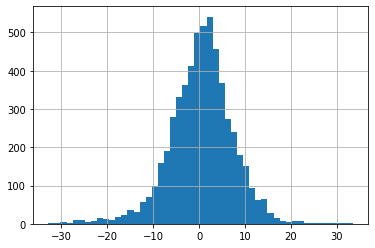
df['COPP'].hist(bins=50)
<AxesSubplot:>
#https://github.com/matplotlib/mplfinance
#this package help visualize financial data
import mplfinance as mpf
import matplotlib.colors as mcolors

# all_colors = list(mcolors.CSS4_COLORS.keys())#"CSS Colors"
# all_colors = list(mcolors.TABLEAU_COLORS.keys()) # "Tableau Palette",
all_colors = ['dodgerblue', 'firebrick','limegreen','skyblue','lightgreen',  'navy','yellow','plum',  'yellowgreen']
# all_colors = list(mcolors.BASE_COLORS.keys()) #"Base Colors",


#https://github.com/matplotlib/mplfinance/issues/181#issuecomment-667252575
#list of colors: https://matplotlib.org/stable/gallery/color/named_colors.html
#https://github.com/matplotlib/mplfinance/blob/master/examples/styles.ipynb

def make_3panels2(main_data, mid_panel, chart_type='candle', names=None,
                  figratio=(14,9), fill_weights = (0, 0)):
    """
    main chart type: default is candle. alternatives: ohlc, line

    example:
    start = 200

    names = {'main_title': 'MAMA: MESA Adaptive Moving Average',
             'sub_tile': 'S&P 500 (^GSPC)', 'y_tiles': ['price', 'Volume [$10^{6}$]']}


    make_candle(df.iloc[-start:, :5], df.iloc[-start:][['MAMA', 'FAMA']], names = names)

    """

    style = mpf.make_mpf_style(base_mpf_style='yahoo',  #charles
                               base_mpl_style = 'seaborn-whitegrid',
#                                marketcolors=mpf.make_marketcolors(up="r", down="#0000CC",inherit=True),
                               gridcolor="whitesmoke",
                               gridstyle="--", #or None, or - for solid
                               gridaxis="both",
                               edgecolor = 'whitesmoke',
                               facecolor = 'white', #background color within the graph edge
                               figcolor = 'white', #background color outside of the graph edge
                               y_on_right = False,
                               rc =  {'legend.fontsize': 'small',#or number
                                      #'figure.figsize': (14, 9),
                                     'axes.labelsize': 'small',
                                     'axes.titlesize':'small',
                                     'xtick.labelsize':'small',#'x-small', 'small','medium','large'
                                     'ytick.labelsize':'small'
                                     },
                              )

    if (chart_type is None) or (chart_type not in ['ohlc', 'line', 'candle', 'hollow_and_filled']):
        chart_type = 'candle'
    len_dict = {'candle':2, 'ohlc':3, 'line':1, 'hollow_and_filled':2}

    kwargs = dict(type=chart_type, figratio=figratio, volume=True, volume_panel=2,
                  panel_ratios=(4,2,1), tight_layout=True, style=style, returnfig=True)

    if names is None:
        names = {'main_title': '', 'sub_tile': ''}


    added_plots = { }

    fb_bbands2_ = dict(y1=fill_weights[0]*np.ones(mid_panel.shape[0]),
                      y2=fill_weights[1]*np.ones(mid_panel.shape[0]),color="lightskyblue",alpha=0.1,interpolate=True)
    fb_bbands2_['panel'] = 1

    fb_bbands= [fb_bbands2_]


    i = 0
    for name_, data_ in mid_panel.iteritems():
        added_plots[name_] = mpf.make_addplot(data_, panel=1, width=1, color=all_colors[i], secondary_y=False)
        i = i + 1


    fig, axes = mpf.plot(main_data,  **kwargs,
                         addplot=list(added_plots.values()),
                         fill_between=fb_bbands)
    # add a new suptitle
    fig.suptitle(names['main_title'], y=1.05, fontsize=12, x=0.1285)

    axes[0].set_title(names['sub_tile'], fontsize=10, style='italic',  loc='left')
#     axes[2].set_ylabel('WAVEPM10')

#     axes[0].set_ylabel(names['y_tiles'][0])
#     axes[2].set_ylabel(names['y_tiles'][1])
    return fig, axes
start = -1200
end = df.shape[0]

names = {'main_title': f'{ticker}',
         'sub_tile': f'Coppock Curve is a momentum indicator to identify major market trend direction for long-term trading strategies.'}


aa_, bb_ = make_3panels2(df.iloc[start:end][['Open', 'High', 'Low', 'Close', 'Volume']],
             df.iloc[start:end][['COPP']],
             chart_type='hollow_and_filled',names = names,
                         fill_weights = (-20, 20))