Awesome Oscillator (AO)
References
Definition
- The Awesome Oscillator is an indicator used to measure market momentum created by Bill Williams.
- AO calculates the difference of a 34 Period and 5 Period Simple Moving Averages.
- The Simple Moving Averages that are used are not calculated using closing price but rather each bar’s midpoints.
- AO is generally used to affirm trends or to anticipate possible reversals.
Calculation
- MP = (High + Low)/2
- Fast SMA = 5 periods Simple Moving Average of MP
- Slow SMA = 34 periods Simple Moving Average of MP
- AO = Fast SMA - Slow SMA
Read the indicator
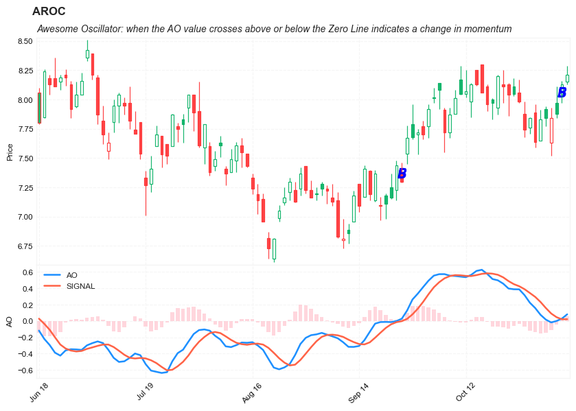
- The Awesome Oscillator is designed to have values that fluctuate above and below a Zero Line.
- The generated values are plotted as a histogram of red and green bars.
- A bar is green when its value is higher than the previous bar.
- A red bar indicates that a bar is lower than the previous bar.
- When AO’s values are above the Zero Line, this indicates that the short term period is trending higher than the long term period.
-
When AO’s values are below the Zero Line, the short term period is trending lower than the Longer term period. This information can be used for a variety of signals.
- Zero Line Cross: when the AO value crosses above or below the Zero Line indicates a change in momentum.
- When AO crosses above the Zero Line, short term momentum is now rising faster than the long term momentum. This can present a bullish buying opportunity.
- When AO crosses below the Zero Line, short term momentum is now falling faster then the long term momentum. This can present a bearish selling opportunity.
- Twin Peaks: Twin Peaks is a method which considers the differences between two peaks on the same side of the Zero Line.
- A Bullish Twin Peaks setup occurs when there are two peaks below the Zero Line. The second peak is higher than the first peak and followed by a green bar. The trough between the two peaks must remain below the Zero Line.
- A Bearish Twin Peaks setup occurs when there are two beaks above the Zero Line. The second peak is lower than the first peak and followed by a red bar. The trough between both peaks must remain above the Zero Line for the duration.
- Saucer: The Saucer method looks for changes in three consecutive bars, all on the same side of the Zero Line.
- A Bullish Saucer setup occurs when the AO is above the Zero Line. It entails two consecutive red bars (with the second bar being lower than the first bar) being followed by a green Bar.
- A Bearish Saucer setup occurs when the AO is below the Zero Line. It entails two consecutive green bars (with the second bar being higher than the first bar) being followed by a red bar.
Load basic packages
import pandas as pd
import numpy as np
import os
import gc
import copy
from pathlib import Path
from datetime import datetime, timedelta, time, date
#this package is to download equity price data from yahoo finance
#the source code of this package can be found here: https://github.com/ranaroussi/yfinance/blob/main
import yfinance as yf
pd.options.display.max_rows = 100
pd.options.display.max_columns = 100

import warnings
warnings.filterwarnings("ignore")

import pytorch_lightning as pl
random_seed=1234
pl.seed_everything(random_seed)
Global seed set to 1234


1234
#S&P 500 (^GSPC),  Dow Jones Industrial Average (^DJI), NASDAQ Composite (^IXIC)
#Russell 2000 (^RUT), Crude Oil Nov 21 (CL=F), Gold Dec 21 (GC=F)
#Treasury Yield 10 Years (^TNX)

#benchmark_tickers = ['^GSPC', '^DJI', '^IXIC', '^RUT',  'CL=F', 'GC=F', '^TNX']

benchmark_tickers = ['^GSPC']
tickers = benchmark_tickers + ['GSK', 'NVO', 'AROC']
#https://github.com/ranaroussi/yfinance/blob/main/yfinance/base.py
#     def history(self, period="1mo", interval="1d",
#                 start=None, end=None, prepost=False, actions=True,
#                 auto_adjust=True, back_adjust=False,
#                 proxy=None, rounding=False, tz=None, timeout=None, **kwargs):

dfs = {}

for ticker in tickers:
    cur_data = yf.Ticker(ticker)
    hist = cur_data.history(period="max", start='2000-01-01')
    print(datetime.now(), ticker, hist.shape, hist.index.min(), hist.index.max())
    dfs[ticker] = hist
2022-08-26 19:06:58.701867 ^GSPC (5700, 7) 1999-12-31 00:00:00 2022-08-25 00:00:00
2022-08-26 19:06:59.073368 GSK (5700, 7) 1999-12-31 00:00:00 2022-08-25 00:00:00
2022-08-26 19:06:59.544649 NVO (5700, 7) 1999-12-31 00:00:00 2022-08-25 00:00:00
2022-08-26 19:06:59.840465 AROC (3781, 7) 2007-08-21 00:00:00 2022-08-25 00:00:00
ticker = 'AROC'
dfs[ticker].tail(5)
| Open | High | Low | Close | Volume | Dividends | Stock Splits | |
|---|---|---|---|---|---|---|---|
| Date | |||||||
| 2022-08-19 | 7.75 | 7.75 | 7.62 | 7.62 | 569100 | 0.0 | 0 |
| 2022-08-22 | 7.59 | 7.68 | 7.50 | 7.62 | 753700 | 0.0 | 0 |
| 2022-08-23 | 7.74 | 7.90 | 7.71 | 7.80 | 732200 | 0.0 | 0 |
| 2022-08-24 | 7.78 | 7.95 | 7.74 | 7.92 | 673800 | 0.0 | 0 |
| 2022-08-25 | 7.95 | 8.00 | 7.84 | 7.92 | 857000 | 0.0 | 0 |
Define Awesome Oscillator (AO) calculation function
#https://github.com/peerchemist/finta/blob/af01fa594995de78f5ada5c336e61cd87c46b151/finta/finta.py

def cal_ao(ohlc: pd.DataFrame, slow_period: int = 34, fast_period: int = 5, signal: int = 9,) -> pd.Series:

    """
    Awesome Oscillator is an indicator used to measure market momentum.
    AO calculates the difference of a 34 Period and 5 Period Simple Moving Averages.
    The Simple Moving Averages that are used are not calculated using closing price but rather each bar's midpoints.
    AO is generally used to affirm trends or to anticipate possible reversals.

    1. MP = (High + Low)/2
    2. Fast SMA = 5 periods Simple Moving Average of MP
    3. Slow SMA = 34 periods Simple Moving Average of MP
    4. AO = Fast SMA - Slow SMA


    """
    ohlc = ohlc.copy()
    ohlc.columns = [c.lower() for c in ohlc.columns]

    mp = (ohlc["high"] + ohlc["low"]) / 2

    slow = pd.Series(mp.rolling(window=slow_period).mean(), name="slow_AO")
    fast = pd.Series(mp.rolling(window=fast_period).mean(), name="fast_AO")

    AO = pd.Series(fast - slow, name="AO")
    AO_signal = pd.Series(
        AO.rolling(window=fast_period).mean(), name="SIGNAL"
    )

    return pd.concat([AO, AO_signal], axis=1)
def get_cross_signal(series: pd.Series, up_buy: int = 1) -> list:
    signals = []
    series.sort_index(ascending=True, inplace=True)


    for i in range(len(series)):
        val = np.nan #not a crossing point

        if series[i]==0:
            if i<2:
                val = np.nan
            else:
                if (series[i-1]<0):
                    val = up_buy
                elif (series[i-1]>0):
                    val = -up_buy
                else:
                    val = np.nan
        else:
            if (i<2)|(i>=len(series)-2):
                val = np.nan
            else:
                if (series[i-1]<0) & (series[i]>0):
                    val = up_buy
                elif (series[i-1]>0) & (series[i]<0):
                    val = -up_buy
                else:
                    val = np.nan

        signals.append(val)

    return signals
Calculate Awesome Oscillator (AO)
df = dfs[ticker][['Open', 'High', 'Low', 'Close', 'Volume']]
df = df.round(2)
cal_ao
<function __main__.cal_ao(ohlc: pandas.core.frame.DataFrame, slow_period: int = 34, fast_period: int = 5, signal: int = 9) -> pandas.core.series.Series>
df_ta = cal_ao(df, slow_period=34, fast_period=5, signal= 9)
df = df.merge(df_ta, left_index = True, right_index = True, how='inner' )

del df_ta
gc.collect()
122
signals = get_cross_signal(df['AO'], 1)
df['AO_BS'] = signals
df['B'] = df['AO_BS']*(df['High']+df['Low'])/2
df['S'] = df['AO_BS']*(df['High']+df['Low'])/2
display(df.head(5))
display(df.tail(5))
| Open | High | Low | Close | Volume | AO | SIGNAL | AO_BS | B | S | |
|---|---|---|---|---|---|---|---|---|---|---|
| Date | ||||||||||
| 2007-08-21 | 50.01 | 50.86 | 49.13 | 49.44 | 1029100 | NaN | NaN | NaN | NaN | NaN |
| 2007-08-22 | 48.50 | 50.70 | 47.78 | 49.29 | 996500 | NaN | NaN | NaN | NaN | NaN |
| 2007-08-23 | 49.76 | 49.82 | 47.56 | 48.03 | 742700 | NaN | NaN | NaN | NaN | NaN |
| 2007-08-24 | 47.93 | 48.77 | 47.87 | 48.58 | 416000 | NaN | NaN | NaN | NaN | NaN |
| 2007-08-27 | 48.56 | 48.81 | 46.85 | 47.47 | 447000 | NaN | NaN | NaN | NaN | NaN |
| Open | High | Low | Close | Volume | AO | SIGNAL | AO_BS | B | S | |
|---|---|---|---|---|---|---|---|---|---|---|
| Date | ||||||||||
| 2022-08-19 | 7.75 | 7.75 | 7.62 | 7.62 | 569100 | -0.157353 | -0.157476 | NaN | NaN | NaN |
| 2022-08-22 | 7.59 | 7.68 | 7.50 | 7.62 | 753700 | -0.162029 | -0.148806 | NaN | NaN | NaN |
| 2022-08-23 | 7.74 | 7.90 | 7.71 | 7.80 | 732200 | -0.153294 | -0.148265 | NaN | NaN | NaN |
| 2022-08-24 | 7.78 | 7.95 | 7.74 | 7.92 | 673800 | -0.107882 | -0.143159 | NaN | NaN | NaN |
| 2022-08-25 | 7.95 | 8.00 | 7.84 | 7.92 | 857000 | -0.069824 | -0.130076 | NaN | NaN | NaN |
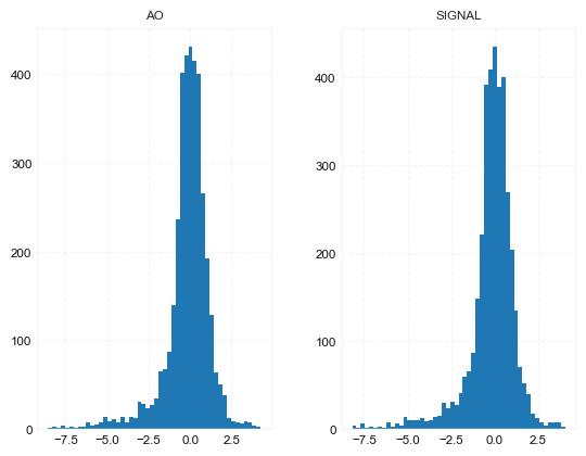
df[['AO', 'SIGNAL']].hist(bins=50)
array([[<AxesSubplot:title={'center':'AO'}>,
        <AxesSubplot:title={'center':'SIGNAL'}>]], dtype=object)
#https://github.com/matplotlib/mplfinance
#this package help visualize financial data
import mplfinance as mpf
import matplotlib.colors as mcolors

# all_colors = list(mcolors.CSS4_COLORS.keys())#"CSS Colors"
all_colors = list(mcolors.TABLEAU_COLORS.keys()) # "Tableau Palette",
# all_colors = list(mcolors.BASE_COLORS.keys()) #"Base Colors",


#https://github.com/matplotlib/mplfinance/issues/181#issuecomment-667252575
#list of colors: https://matplotlib.org/stable/gallery/color/named_colors.html
#https://github.com/matplotlib/mplfinance/blob/master/examples/styles.ipynb

def plot_macd(main_data, add_data, mid_panel, chart_type='candle', names=None,
                  figratio=(14,9)):


    style = mpf.make_mpf_style(base_mpf_style='yahoo',  #charles
                               base_mpl_style = 'seaborn-whitegrid',
#                                marketcolors=mpf.make_marketcolors(up="r", down="#0000CC",inherit=True),
                               gridcolor="whitesmoke",
                               gridstyle="--", #or None, or - for solid
                               gridaxis="both",
                               edgecolor = 'whitesmoke',
                               facecolor = 'white', #background color within the graph edge
                               figcolor = 'white', #background color outside of the graph edge
                               y_on_right = False,
                               rc =  {'legend.fontsize': 'small',#or number
                                      #'figure.figsize': (14, 9),
                                     'axes.labelsize': 'small',
                                     'axes.titlesize':'small',
                                     'xtick.labelsize':'small',#'x-small', 'small','medium','large'
                                     'ytick.labelsize':'small'
                                     },
                              )

    if (chart_type is None) or (chart_type not in ['ohlc', 'line', 'candle', 'hollow_and_filled']):
        chart_type = 'candle'
    len_dict = {'candle':2, 'ohlc':3, 'line':1, 'hollow_and_filled':2}

    kwargs = dict(type=chart_type, figratio=figratio, volume=False,
                  panel_ratios=(4,2), tight_layout=True, style=style, returnfig=True)

    if names is None:
        names = {'main_title': '', 'sub_tile': ''}


    added_plots = {
        'S':  mpf.make_addplot(add_data['S'], panel=0, color='blue', type='scatter', marker=r'${S}$' , markersize=100, secondary_y=False),
        'B':  mpf.make_addplot(add_data['B'], panel=0, color='blue', type='scatter', marker=r'${B}$' , markersize=100, secondary_y=False),

        'AO': mpf.make_addplot(mid_panel['AO'], panel=1, color='dodgerblue', secondary_y=False),
        'SIGNAL': mpf.make_addplot(mid_panel['SIGNAL'], panel=1, color='tomato', secondary_y=False),
        'AO-SIGNAL': mpf.make_addplot(mid_panel['AO']-mid_panel['SIGNAL'], type='bar',width=0.7,panel=1, color="pink",alpha=0.65,secondary_y=False),
    }


    fig, axes = mpf.plot(main_data,  **kwargs,
                         addplot=list(added_plots.values()),
                        )
    # add a new suptitle
    fig.suptitle(names['main_title'], y=1.05, fontsize=12, x=0.128)

    axes[0].set_title(names['sub_tile'], fontsize=10, style='italic',  loc='left')


    #set legend

    axes[2].legend([None]*2)
    handles = axes[2].get_legend().legendHandles
#     print(handles)
    axes[2].legend(handles=handles,labels=['AO', 'SIGNAL'])
    #axes[2].set_title('AO', fontsize=10, style='italic',  loc='left')
    axes[2].set_ylabel('AO')


#     axes[0].set_ylabel(names['y_tiles'][0])
    return fig, axes
start = -300
end = -200#df.shape[0]

names = {'main_title': f'{ticker}',
         'sub_tile': 'Awesome Oscillator: when the AO value crosses above or below the Zero Line indicates a change in momentum'}


aa_, bb_ = plot_macd(df.iloc[start:end][['Open', 'High', 'Low', 'Close', 'Volume']],
             df.iloc[start:end][['B', 'S']],
             df.iloc[start:end][['AO', 'SIGNAL']],
             chart_type='hollow_and_filled',
                     names = names,
                    )