Bollinger Bands Introduction

References

• tradingview: Bollinger Bands (BB)
• tradingview: Bollinger Bands %B
• tradingview: Bollinger Bands Width (BBW)

Bollinger Bands (BB)

Definition

• Bollinger Bands (BB) were created by John Bollinger in the early 1980’s to fill the need to visualize changes in volatility.
• Bollinger Bands consist of three lines:
  • the middle line is 20-day Simple Moving Average (SMA). (20 days can be replaced by other periods, such as 10 days)
  • the upper line is several - typically 2 - standard deviations above the middle line
  • the lower line is same number of standard deviations below the middle line

Calculation

---

• Middle Band – 20 Day Simple Moving Average
• Upper Band – 20 Day Simple Moving Average + (Standard Deviation x 2)
• Lower Band – 20 Day Simple Moving Average - (Standard Deviation x 2)

---

• MOBO bands are based on a zone of 0.80 standard deviation with a 10 period look-back. If the price breaks out of the MOBO band it can signify a trend move or price spike contains 42% of price movements(noise) within bands.

Bollinger Bands %B

Percent Bandwidth (%B)

Definition

• Bollinger Bands %B or Percent Bandwidth (%B) is an indicator derived from the standard Bollinger Bands (BB).
• John Bollinger introduced %B in 2010.

Calculation

%B = (Current Price - Lower Band) / (Upper Band - Lower Band)

Read the indicator

• %B Above 1 = Price is Above the Upper Band
• %B Equal to 1 = Price is at the Upper Band
• %B Above .50 = Price is Above the Middle Line
• %B Below .50 = Price is Below the Middle Line
• %B Equal to 0 = Price is at the Lower Band
• %B Below 0 = Price is Below the Lower Band

Bollinger Bands Width (BBW)

Definition

• Bollinger Bands Width (BBW) is derived from the standard Bollinger Bands.
  • John Bollinger introduced Bollinger Bands Width in 2010.

Calculation - Bollinger Bands Width = (Upper Band - Lower Band) / Middle Band

Load basic packages

import pandas as pd
import numpy as np
import os
import gc
import copy
from pathlib import Path
from datetime import datetime, timedelta, time, date

#this package is to download equity price data from yahoo finance
#the source code of this package can be found here: https://github.com/ranaroussi/yfinance/blob/main
import yfinance as yf

pd.options.display.max_rows = 100
pd.options.display.max_columns = 100

import warnings
warnings.filterwarnings("ignore")

import pytorch_lightning as pl
random_seed=1234
pl.seed_everything(random_seed)

Global seed set to 1234





1234

#S&P 500 (^GSPC),  Dow Jones Industrial Average (^DJI), NASDAQ Composite (^IXIC)
#Russell 2000 (^RUT), Crude Oil Nov 21 (CL=F), Gold Dec 21 (GC=F)
#Treasury Yield 10 Years (^TNX)

#benchmark_tickers = ['^GSPC', '^DJI', '^IXIC', '^RUT',  'CL=F', 'GC=F', '^TNX']

benchmark_tickers = ['^GSPC']
tickers = benchmark_tickers + ['GSK', 'NVO', 'GKOS']

#https://github.com/ranaroussi/yfinance/blob/main/yfinance/base.py
#     def history(self, period="1mo", interval="1d",
#                 start=None, end=None, prepost=False, actions=True,
#                 auto_adjust=True, back_adjust=False,
#                 proxy=None, rounding=False, tz=None, timeout=None, **kwargs):

dfs = {}

for ticker in tickers:
    cur_data = yf.Ticker(ticker)
    hist = cur_data.history(period="max", start='2000-01-01')
    print(datetime.now(), ticker, hist.shape, hist.index.min(), hist.index.max())
    dfs[ticker] = hist

2022-09-09 18:47:27.422799 ^GSPC (5709, 7) 1999-12-31 00:00:00 2022-09-08 00:00:00
2022-09-09 18:47:27.705493 GSK (5709, 7) 1999-12-31 00:00:00 2022-09-08 00:00:00
2022-09-09 18:47:28.061476 NVO (5709, 7) 1999-12-31 00:00:00 2022-09-08 00:00:00
2022-09-09 18:47:28.263999 GKOS (1815, 7) 2015-06-25 00:00:00 2022-09-08 00:00:00

ticker = 'GSK'
dfs[ticker].tail(5)

	Open	High	Low	Close	Volume	Dividends	Stock Splits
Date
2022-09-01	31.830000	31.990000	31.610001	31.690001	12390900	0.0	0.0
2022-09-02	31.600000	31.969999	31.469999	31.850000	8152600	0.0	0.0
2022-09-06	31.650000	31.760000	31.370001	31.469999	5613900	0.0	0.0
2022-09-07	31.209999	31.590000	31.160000	31.490000	4822000	0.0	0.0
2022-09-08	30.910000	31.540001	30.830000	31.510000	6619300	0.0	0.0

Define Bollinger Bands calculation function

#https://github.com/peerchemist/finta/blob/af01fa594995de78f5ada5c336e61cd87c46b151/finta/finta.py#L935
def cal_bbands(ohlc: pd.DataFrame, period: int = 20, column: str = "close", 
               MA: pd.Series = None, std_multiplier: float = 2) -> pd.DataFrame:
    
    """
     Developed by John Bollinger, Bollinger Bands® are volatility bands placed above and below a moving average.
     Volatility is based on the standard deviation, which changes as volatility increases and decreases.
     The bands automatically widen when volatility increases and narrow when volatility decreases.
     This method allows input of some other form of moving average like EMA or KAMA around which BBAND will be formed.
     Pass desired moving average as <MA> argument. For example BBANDS(MA=TA.KAMA(20)).
    

    "MOBO bands are based on a zone of 0.80 standard deviation with a 10 period look-back"
    If the price breaks out of the MOBO band it can signify a trend move or price spike
    Contains 42% of price movements(noise) within bands.
    
    BBANDS(ohlc, period=10, std_multiplier=0.8, column=column)
    
    BBWIDTH: Bandwidth tells how wide the Bollinger Bands are on a normalized basis.
    %b (pronounced 'percent b') is derived from the formula for Stochastics and shows where price is in relation to the bands.
    %b equals 1 at the upper band and 0 at the lower band.
     
     """
    
    ohlc = ohlc.copy(deep=True)
    ohlc.columns = [c.lower() for c in ohlc.columns]
    
    std = ohlc[column].rolling(window=period).std()

    if not isinstance(MA, pd.Series):
        middle_band = pd.Series( ohlc[column].rolling(window=period).mean(), name="BB_MIDDLE")
    else:
        middle_band = pd.Series(MA, name="BB_MIDDLE")

    upper_bb = pd.Series(middle_band + (std_multiplier * std), name="BB_UPPER")
    lower_bb = pd.Series(middle_band - (std_multiplier * std), name="BB_LOWER")
    
    width_bb = pd.Series((upper_bb - lower_bb)/middle_band, name='BBWIDTH')
    
    percent_b = pd.Series(
            (ohlc["close"] - lower_bb) / (upper_bb - lower_bb),
            name="pct_b",
        )
    

    return pd.concat([upper_bb, middle_band, lower_bb, width_bb, percent_b], axis=1)

Calculate Bollinger Bands

df = dfs[ticker][['Open', 'High', 'Low', 'Close', 'Volume']]

df = df.round(2)

cal_bbands

<function __main__.cal_bbands(ohlc: pandas.core.frame.DataFrame, period: int = 20, column: str = 'close', MA: pandas.core.series.Series = None, std_multiplier: float = 2) -> pandas.core.frame.DataFrame>

df_ta = cal_bbands(df, period = 20, column = 'close', std_multiplier=2)
df = df.merge(df_ta, left_index = True, right_index = True, how='inner' )

del df_ta
gc.collect()

122

df_ta = cal_bbands(df, period = 10, column = 'close', std_multiplier=0.8)
df_ta.columns=[f'MOBO_{c}' for c in df_ta.columns]
df = df.merge(df_ta, left_index = True, right_index = True, how='inner' )

del df_ta
gc.collect()

21

display(df.head(5))
display(df.tail(5))

	Open	High	Low	Close	Volume	BB_UPPER	BB_MIDDLE	BB_LOWER	BBWIDTH	pct_b	MOBO_BB_UPPER	MOBO_BB_MIDDLE	MOBO_BB_LOWER	MOBO_BBWIDTH	MOBO_pct_b
Date
1999-12-31	19.60	19.67	19.52	19.56	139400	NaN	NaN	NaN	NaN	NaN	NaN	NaN	NaN	NaN	NaN
2000-01-03	19.58	19.71	19.25	19.45	556100	NaN	NaN	NaN	NaN	NaN	NaN	NaN	NaN	NaN	NaN
2000-01-04	19.45	19.45	18.90	18.95	367200	NaN	NaN	NaN	NaN	NaN	NaN	NaN	NaN	NaN	NaN
2000-01-05	19.21	19.58	19.08	19.58	481700	NaN	NaN	NaN	NaN	NaN	NaN	NaN	NaN	NaN	NaN
2000-01-06	19.38	19.43	18.90	19.30	853800	NaN	NaN	NaN	NaN	NaN	NaN	NaN	NaN	NaN	NaN

	Open	High	Low	Close	Volume	BB_UPPER	BB_MIDDLE	BB_LOWER	BBWIDTH	pct_b	MOBO_BB_UPPER	MOBO_BB_MIDDLE	MOBO_BB_LOWER	MOBO_BBWIDTH	MOBO_pct_b
Date
2022-09-01	31.83	31.99	31.61	31.69	12390900	39.888247	34.9440	29.999753	0.282981	0.170931	33.847434	33.253	32.658566	0.035752	-0.814696
2022-09-02	31.60	31.97	31.47	31.85	8152600	39.017011	34.5310	30.044989	0.259825	0.201182	33.674094	33.032	32.389906	0.038877	-0.420425
2022-09-06	31.65	31.76	31.37	31.47	5613900	38.032892	34.1115	30.190108	0.229916	0.163194	33.455731	32.774	32.092269	0.041602	-0.456390
2022-09-07	31.21	31.59	31.16	31.49	4822000	36.843798	33.7070	30.570202	0.186121	0.146614	33.243774	32.550	31.856226	0.042628	-0.263937
2022-09-08	30.91	31.54	30.83	31.51	6619300	35.993101	33.3890	30.784899	0.155986	0.139223	33.026915	32.348	31.669085	0.041976	-0.117161

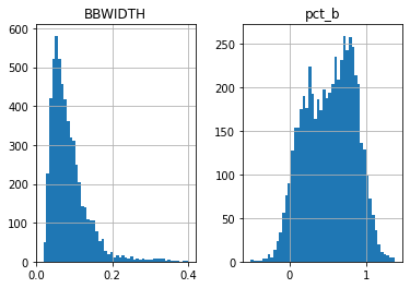
df[['BBWIDTH', 'pct_b']].hist(bins=50)

array([[<AxesSubplot:title={'center':'BBWIDTH'}>,
        <AxesSubplot:title={'center':'pct_b'}>]], dtype=object)

df.columns

Index(['Open', 'High', 'Low', 'Close', 'Volume', 'BB_UPPER', 'BB_MIDDLE',
       'BB_LOWER', 'BBWIDTH', 'pct_b', 'MOBO_BB_UPPER', 'MOBO_BB_MIDDLE',
       'MOBO_BB_LOWER', 'MOBO_BBWIDTH', 'MOBO_pct_b'],
      dtype='object')

import pandas as pd
import numpy as np
import copy
import os
import json

#https://github.com/matplotlib/mplfinance
#this package help visualize financial data
import mplfinance as mpf
import matplotlib.colors as mcolors

all_colors = list(mcolors.CSS4_COLORS.keys())#"CSS Colors"
# all_colors = list(mcolors.TABLEAU_COLORS.keys()) # "Tableau Palette",
# all_colors = list(mcolors.BASE_COLORS.keys()) #"Base Colors",


#https://github.com/matplotlib/mplfinance/issues/181#issuecomment-667252575
#list of colors: https://matplotlib.org/stable/gallery/color/named_colors.html
#https://github.com/matplotlib/mplfinance/blob/master/examples/styles.ipynb
#https://matplotlib.org/stable/gallery/lines_bars_and_markers/marker_reference.html




def make_bbands(main_data, add_data, mid_panel, 
                       chart_type='candle', names=None, 
                       figratio=(14,9), 
                       fill_weights = (0, 0)  ):


    style = mpf.make_mpf_style(base_mpf_style='yahoo',  #charles
                               base_mpl_style = 'seaborn-whitegrid',
#                                marketcolors=mpf.make_marketcolors(up="r", down="#0000CC",inherit=True),
                               gridcolor="whitesmoke", 
                               gridstyle="--", #or None, or - for solid
                               gridaxis="both", 
                               edgecolor = 'whitesmoke',
                               facecolor = 'white', #background color within the graph edge
                               figcolor = 'white', #background color outside of the graph edge
                               y_on_right = False,
                               rc =  {'legend.fontsize': 'small',#or number
                                      'figure.figsize': (16, 16),
                                     'axes.labelsize': 'small',
                                     'axes.titlesize':'small',
                                     'xtick.labelsize':'small',#'x-small', 'small','medium','large'
                                     'ytick.labelsize':'small'
                                     }, 
                              )   

    if (chart_type is None) or (chart_type not in ['ohlc', 'line', 'candle', 'hollow_and_filled']):
        chart_type = 'candle'
    len_dict = {'candle':2, 'ohlc':3, 'line':1, 'hollow_and_filled':2}    
        
    kwargs = dict(type=chart_type, figratio=figratio, volume=False, 
                  panel_ratios=(6, 2, 2), tight_layout=True, style=style, returnfig=True)
    
    if names is None:
        names = {'main_title': '', 'sub_tile': ''}


    added_plots = { 
        'BB_UPPER':  mpf.make_addplot(add_data['BB_UPPER'], panel=0, color='dodgerblue', width=1, secondary_y=False),
        'BB_LOWER':  mpf.make_addplot(add_data['BB_LOWER'], panel=0, color='green', width=1, secondary_y=False), 
        'BB_MIDDLE':  mpf.make_addplot(add_data['BB_MIDDLE'], panel=0, color='tomato', width=1, secondary_y=False), 

        'BBWIDTH':  mpf.make_addplot(mid_panel['BBWIDTH'], panel=1, color='dodgerblue', width=1, secondary_y=False), 
        
        '%B':  mpf.make_addplot(mid_panel['pct_b'], panel=2, color='dodgerblue', width=1, secondary_y=False), 
        
    }
    
    fb_1 = dict(y1=add_data['BB_UPPER'].values,
                      y2=add_data['BB_LOWER'].values,color="lightskyblue",alpha=0.1,interpolate=True)
    fb_1['panel'] = 0
    
        
    fb_2 = dict(y1=fill_weights[0]*np.ones(mid_panel.shape[0]),
                      y2=fill_weights[1]*np.ones(mid_panel.shape[0]),color="lightskyblue",alpha=0.1,interpolate=True)
    fb_2['panel'] = 1
    
        
    fb_3 = dict(y1=0*np.ones(mid_panel.shape[0]),
                      y2=1*np.ones(mid_panel.shape[0]),color="lightskyblue",alpha=0.1,interpolate=True)
    fb_3['panel'] = 2
    
    fb_bbands= [fb_1, fb_2, fb_3 ]
 

    fig, axes = mpf.plot(main_data,  **kwargs,
                         addplot=list(added_plots.values()), 
                         fill_between=fb_bbands, 
                         )
    # add a new suptitle
    fig.suptitle(names['main_title'], y=1.05, fontsize=12, x=0.1295)

    axes[0].set_title(names['sub_tile'], fontsize=9, style='italic',  loc='left')
    axes[0].legend([None]*5)
    handles = axes[0].get_legend().legendHandles
    axes[0].legend(handles=handles[2:],labels=['BB_UPPER', 'BB_LOWER', 'BB_MIDDLE'])
    
    axes[2].set_title('BBWIDTH', fontsize=9, style='italic',  loc='left')
    #axes[2].set_ylabel('CCI') 
    axes[2].legend([None]*1)
    handles = axes[2].get_legend().legendHandles
    axes[2].legend(handles=handles,labels=['BBWIDTH'])
    
    axes[4].set_title('%B', fontsize=9, style='italic',  loc='left')
    #axes[4].set_ylabel('Decycler oscillator')
    axes[4].legend([None]*3)
    handles = axes[4].get_legend().legendHandles
    axes[4].legend(handles=handles,labels=['%B'])   
     
    
    return fig, axes

start = -300
end = df.shape[0]

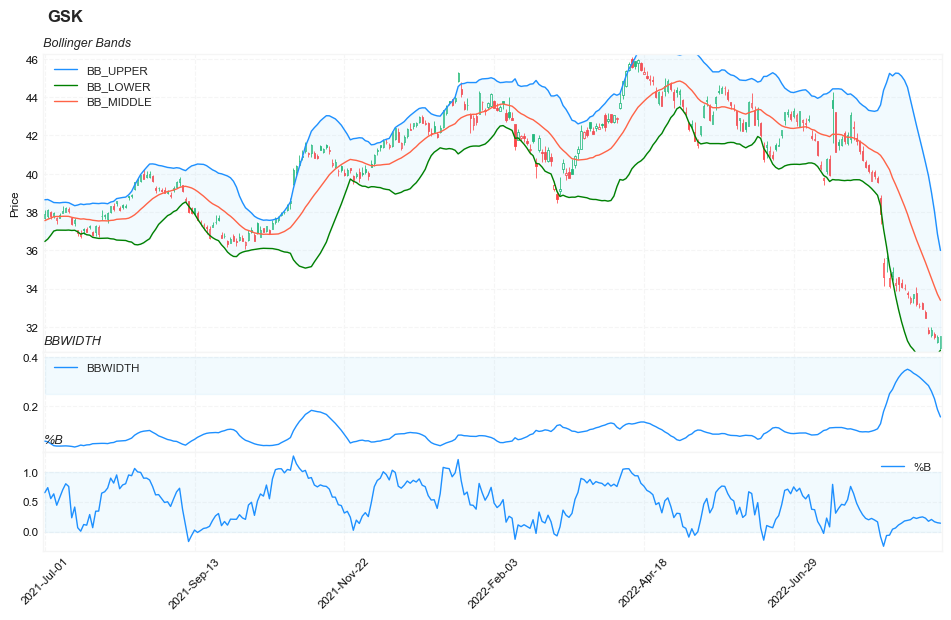
names = {'main_title': f'{ticker}', 
         'sub_tile': 'Bollinger Bands'}


aa_, bb_ = make_bbands(df.iloc[start:end][['Open', 'High', 'Low', 'Close', 'Volume']], 
                         df.iloc[start:end][['BB_UPPER', 'BB_MIDDLE','BB_LOWER']], 
                         df.iloc[start:end][['BBWIDTH', 'pct_b']], 
                         chart_type='hollow_and_filled',
                         names = names, 
                           figratio=(18,10), 
                           fill_weights = (0.25, 0.4) 
                        
                        )