BRAR
References
Definition
Emotional index (BRAR) is also called popularity intention index. It consists of two indicators: popularity index (AR) and willingness index (BR). Both the AR indicator and the BR indicator are technical indicators based on the analysis of historical stock prices.
- the BRAR indicator is 100-centric. When BR around 100 indicates the sentiment of the market is in a very balanced state.
- when the BRAR starts to fluctuate, it can rise above 200 or drop below 80.
Read the indicator
- AR indicator can be used alone, and BR indicator needs to be used in conjunction with AR indicators in order to be effective.
- BRAR is not suitable for capturing a large bottom, but it can be used to capture a local bottom.
Buy signals:
- BR line normally runs above AR line, when BR crosses AR and runs below AR line
- BR<40 and AR<60
- BR <AR and AR <50
- BR <AR and BR <100
Sell signals
- BR>400 and AR>180
- BR rapadily increases but AR stays flat or slightly drops
Load basic packages
import pandas as pd
import numpy as np
import os
import gc
import copy
from pathlib import Path
from datetime import datetime, timedelta, time, date
#this package is to download equity price data from yahoo finance
#the source code of this package can be found here: https://github.com/ranaroussi/yfinance/blob/main
import yfinance as yf
pd.options.display.max_rows = 100
pd.options.display.max_columns = 100

import warnings
warnings.filterwarnings("ignore")

import pytorch_lightning as pl
random_seed=1234
pl.seed_everything(random_seed)
Global seed set to 1234


1234
#S&P 500 (^GSPC),  Dow Jones Industrial Average (^DJI), NASDAQ Composite (^IXIC)
#Russell 2000 (^RUT), Crude Oil Nov 21 (CL=F), Gold Dec 21 (GC=F)
#Treasury Yield 10 Years (^TNX)

#benchmark_tickers = ['^GSPC', '^DJI', '^IXIC', '^RUT',  'CL=F', 'GC=F', '^TNX']

benchmark_tickers = ['^GSPC']
tickers = benchmark_tickers + ['GSK', 'NVO', 'GKOS']
#https://github.com/ranaroussi/yfinance/blob/main/yfinance/base.py
#     def history(self, period="1mo", interval="1d",
#                 start=None, end=None, prepost=False, actions=True,
#                 auto_adjust=True, back_adjust=False,
#                 proxy=None, rounding=False, tz=None, timeout=None, **kwargs):

dfs = {}

for ticker in tickers:
    cur_data = yf.Ticker(ticker)
    hist = cur_data.history(period="max", start='2000-01-01')
    print(datetime.now(), ticker, hist.shape, hist.index.min(), hist.index.max())
    dfs[ticker] = hist
2022-09-10 21:31:52.358741 ^GSPC (5710, 7) 1999-12-31 00:00:00 2022-09-09 00:00:00
2022-09-10 21:31:52.676873 GSK (5710, 7) 1999-12-31 00:00:00 2022-09-09 00:00:00
2022-09-10 21:31:53.016940 NVO (5710, 7) 1999-12-31 00:00:00 2022-09-09 00:00:00
2022-09-10 21:31:53.171193 GKOS (1816, 7) 2015-06-25 00:00:00 2022-09-09 00:00:00
ticker = 'GKOS'
dfs[ticker].tail(5)
| Open | High | Low | Close | Volume | Dividends | Stock Splits | |
|---|---|---|---|---|---|---|---|
| Date | |||||||
| 2022-09-02 | 49.590000 | 50.900002 | 48.419998 | 48.830002 | 650900 | 0 | 0 |
| 2022-09-06 | 49.200001 | 49.200001 | 47.630001 | 48.099998 | 334400 | 0 | 0 |
| 2022-09-07 | 52.759998 | 60.919998 | 51.490002 | 57.009998 | 4560500 | 0 | 0 |
| 2022-09-08 | 56.439999 | 59.599998 | 56.439999 | 58.380001 | 1106900 | 0 | 0 |
| 2022-09-09 | 58.369999 | 58.529999 | 55.860001 | 56.299999 | 1291100 | 0 | 0 |
Define BRAR calculation function
def BRAR(OPEN,CLOSE,HIGH,LOW,M1=26):                 #BRAR-ARBR 情绪指标
    AR = SUM(HIGH - OPEN, M1) / SUM(OPEN - LOW, M1) * 100
    BR = SUM(MAX(0, HIGH - REF(CLOSE, 1)), M1) / SUM(MAX(0, REF(CLOSE, 1) - LOW), M1) * 100
    return AR, BR
def cal_brar(ohlc: pd.DataFrame, period: int = 26) -> pd.DataFrame:
    """
    BUY: AR<60 BR<40
    SELL: BR>400, AR>180

    reference:

    https://github.com/mpquant/MyTT/blob/ea4f14857ecc46a3739a75ce2e6974b9057a6102/MyTT.py
    https://github.com/twopirllc/pandas-ta/blob/2a24fdc1b69110332db39eda9723a628f75eaf7a/pandas_ta/momentum/brar.py

    """

    ohlc = ohlc.copy()
    ohlc.columns = [c.lower() for c in ohlc.columns]

    h, l, o, c = ohlc["high"], ohlc["low"], ohlc["open"], ohlc["close"]
    c1 = c.shift(1)

    a0 = (h-o).rolling(period).sum()
    a1 = (o-l).rolling(period).sum()
    ar = a0/a1*100

    b0 = (h - c1).apply(lambda x: max(0, x)).rolling(period).sum()
    b1 = (c1 - l).apply(lambda x: max(0, x)).rolling(period).sum()
    br = b0/b1*100

    return pd.DataFrame(data={'AR': ar.values, 'BR': br.values}, index=ohlc.index)
Calculate BRAR
df = dfs[ticker][['Open', 'High', 'Low', 'Close', 'Volume']]
df = df.round(2)
help(cal_brar)
Help on function cal_brar in module __main__:

cal_brar(ohlc: pandas.core.frame.DataFrame, period: int = 26) -> pandas.core.frame.DataFrame
    BUY: AR<60 BR<40
    SELL: BR>400, AR>180

    reference:

    https://github.com/mpquant/MyTT/blob/ea4f14857ecc46a3739a75ce2e6974b9057a6102/MyTT.py
    https://github.com/twopirllc/pandas-ta/blob/2a24fdc1b69110332db39eda9723a628f75eaf7a/pandas_ta/momentum/brar.py
df_ta = cal_brar(df, period = 14)
df = df.merge(df_ta, left_index = True, right_index = True, how='inner' )

del df_ta
gc.collect()
122
#     BUY: AR<60 BR<40
#     SELL: BR>400, AR>180

df['B'] = ((df["AR"]<60) & (df["BR"]<40)).astype(int)*(df['High']+df['Low'])/2
df['S'] = ((df["AR"]>180) & (df["BR"]>400)).astype(int)*(df['High']+df['Low'])/2
display(df.head(5))
display(df.tail(5))
| Open | High | Low | Close | Volume | AR | BR | B | S | |
|---|---|---|---|---|---|---|---|---|---|
| Date | |||||||||
| 2015-06-25 | 29.11 | 31.95 | 28.00 | 31.22 | 7554700 | NaN | NaN | 0.0 | 0.0 |
| 2015-06-26 | 30.39 | 30.39 | 27.51 | 28.00 | 1116500 | NaN | NaN | 0.0 | 0.0 |
| 2015-06-29 | 27.70 | 28.48 | 27.51 | 28.00 | 386900 | NaN | NaN | 0.0 | 0.0 |
| 2015-06-30 | 27.39 | 29.89 | 27.39 | 28.98 | 223900 | NaN | NaN | 0.0 | 0.0 |
| 2015-07-01 | 28.83 | 29.00 | 27.87 | 28.00 | 150000 | NaN | NaN | 0.0 | 0.0 |
| Open | High | Low | Close | Volume | AR | BR | B | S | |
|---|---|---|---|---|---|---|---|---|---|
| Date | |||||||||
| 2022-09-02 | 49.59 | 50.90 | 48.42 | 48.83 | 650900 | 48.783455 | 57.727550 | 0.0 | 0.0 |
| 2022-09-06 | 49.20 | 49.20 | 47.63 | 48.10 | 334400 | 45.229469 | 59.610553 | 0.0 | 0.0 |
| 2022-09-07 | 52.76 | 60.92 | 51.49 | 57.01 | 4560500 | 96.770186 | 161.901306 | 0.0 | 0.0 |
| 2022-09-08 | 56.44 | 59.60 | 56.44 | 58.38 | 1106900 | 116.763754 | 187.993921 | 0.0 | 0.0 |
| 2022-09-09 | 58.37 | 58.53 | 55.86 | 56.30 | 1291100 | 110.436893 | 180.231716 | 0.0 | 0.0 |
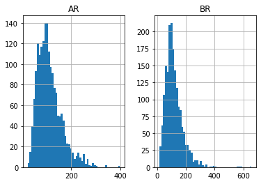
df[['AR','BR']].hist(bins=50)
array([[<AxesSubplot:title={'center':'AR'}>,
        <AxesSubplot:title={'center':'BR'}>]], dtype=object)
#https://github.com/matplotlib/mplfinance
#this package help visualize financial data
import mplfinance as mpf
import matplotlib.colors as mcolors

# all_colors = list(mcolors.CSS4_COLORS.keys())#"CSS Colors"
all_colors = list(mcolors.TABLEAU_COLORS.keys()) # "Tableau Palette",
# all_colors = list(mcolors.BASE_COLORS.keys()) #"Base Colors",


#https://github.com/matplotlib/mplfinance/issues/181#issuecomment-667252575
#list of colors: https://matplotlib.org/stable/gallery/color/named_colors.html
#https://github.com/matplotlib/mplfinance/blob/master/examples/styles.ipynb

def plot_3panels(main_data, add_data=None, mid_panel=None, chart_type='candle', names=None,
                  figratio=(14,9)):


    style = mpf.make_mpf_style(base_mpf_style='yahoo',  #charles
                               base_mpl_style = 'seaborn-whitegrid',
#                                marketcolors=mpf.make_marketcolors(up="r", down="#0000CC",inherit=True),
                               gridcolor="whitesmoke",
                               gridstyle="--", #or None, or - for solid
                               gridaxis="both",
                               edgecolor = 'whitesmoke',
                               facecolor = 'white', #background color within the graph edge
                               figcolor = 'white', #background color outside of the graph edge
                               y_on_right = False,
                               rc =  {'legend.fontsize': 'small',#or number
                                      #'figure.figsize': (14, 9),
                                     'axes.labelsize': 'small',
                                     'axes.titlesize':'small',
                                     'xtick.labelsize':'small',#'x-small', 'small','medium','large'
                                     'ytick.labelsize':'small'
                                     },
                              )

    if (chart_type is None) or (chart_type not in ['ohlc', 'line', 'candle', 'hollow_and_filled']):
        chart_type = 'candle'
    len_dict = {'candle':2, 'ohlc':3, 'line':1, 'hollow_and_filled':2}

    kwargs = dict(type=chart_type, figratio=figratio, volume=False,
                  panel_ratios=(4,2), tight_layout=True, style=style, returnfig=True)

    if names is None:
        names = {'main_title': '', 'sub_tile': ''}


    added_plots = {
        'S':  mpf.make_addplot(add_data['S'], panel=0, color='blue', type='scatter', marker=r'${S}$' , markersize=100, secondary_y=False),
        'B':  mpf.make_addplot(add_data['B'], panel=0, color='blue', type='scatter', marker=r'${B}$' , markersize=100, secondary_y=False),

        'AR': mpf.make_addplot(mid_panel['AR'], panel=1, color='dodgerblue', secondary_y=False),
        'BR': mpf.make_addplot(mid_panel['BR'], panel=1, color='tomato', secondary_y=False),
#         'AO-SIGNAL': mpf.make_addplot(mid_panel['AO']-mid_panel['SIGNAL'], type='bar',width=0.7,panel=1, color="pink",alpha=0.65,secondary_y=False),
    }


    fig, axes = mpf.plot(main_data,  **kwargs,
                         addplot=list(added_plots.values()),
                        )
    # add a new suptitle
    fig.suptitle(names['main_title'], y=1.05, fontsize=12, x=0.128)

    axes[0].set_title(names['sub_tile'], fontsize=10, style='italic',  loc='left')


    #set legend

    axes[2].legend([None]*2)
    handles = axes[2].get_legend().legendHandles
#     print(handles)
    axes[2].legend(handles=handles,labels=['AR', 'BR'])
    #axes[2].set_title('AO', fontsize=10, style='italic',  loc='left')
    axes[2].set_ylabel('BRAR')


#     axes[0].set_ylabel(names['y_tiles'][0])
    return fig, axes
start = -100
end = df.shape[0]
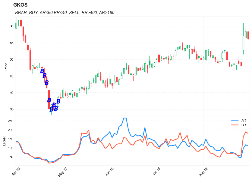
names = {'main_title': f'{ticker}',
'sub_tile': 'BRAR: BUY: AR<60 BR<40; SELL: BR>400, AR>180'}
aa_, bb_ = plot_3panels(df.iloc[start:end][['Open', 'High', 'Low', 'Close', 'Volume']],
df.iloc[start:end][['B', 'S']],
df.iloc[start:end][['AR', 'BR']],
chart_type='hollow_and_filled',
names = names,
)