VAMA: A New Adaptive Moving Average
Reference:
Definition
- The separation of the trend from random fluctuations (noise) is a major objective in technical analysis
- the simple moving average and the exponential moving average are the two most used filters used to achieve this goal
- those two filters use one parameter to control this degree of separation, higher degree of separation involve smoother results but also more lag.
- Lag is defined as the effect of a moving average to show past trends instead of new ones, this effect his unavoidable with causal filters and is a major drawback in decision timing .
- a new adaptive moving average technical indicator (VAMA) aims to provide smooth results as well as providing fast decision timing.
Calculation


Load basic packages
import pandas as pd
import numpy as np
import os
import gc
import copy
from pathlib import Path
from datetime import datetime, timedelta, time, date
#this package is to download equity price data from yahoo finance
#the source code of this package can be found here: https://github.com/ranaroussi/yfinance/blob/main
import yfinance as yf
pd.options.display.max_rows = 100
pd.options.display.max_columns = 100

import warnings
warnings.filterwarnings("ignore")

import pytorch_lightning as pl
random_seed=1234
pl.seed_everything(random_seed)
Global seed set to 1234


1234
#S&P 500 (^GSPC),  Dow Jones Industrial Average (^DJI), NASDAQ Composite (^IXIC)
#Russell 2000 (^RUT), Crude Oil Nov 21 (CL=F), Gold Dec 21 (GC=F)
#Treasury Yield 10 Years (^TNX)

#benchmark_tickers = ['^GSPC', '^DJI', '^IXIC', '^RUT',  'CL=F', 'GC=F', '^TNX']

benchmark_tickers = ['^GSPC']
tickers = benchmark_tickers + ['GSK', 'NVO', 'AROC', 'GKOS']
#https://github.com/ranaroussi/yfinance/blob/main/yfinance/base.py
#     def history(self, period="1mo", interval="1d",
#                 start=None, end=None, prepost=False, actions=True,
#                 auto_adjust=True, back_adjust=False,
#                 proxy=None, rounding=False, tz=None, timeout=None, **kwargs):

dfs = {}

for ticker in tickers:
    cur_data = yf.Ticker(ticker)
    hist = cur_data.history(period="max", start='2000-01-01')
    print(datetime.now(), ticker, hist.shape, hist.index.min(), hist.index.max())
    dfs[ticker] = hist
2022-09-09 19:39:16.539924 ^GSPC (5709, 7) 1999-12-31 00:00:00 2022-09-08 00:00:00
2022-09-09 19:39:16.992681 GSK (5709, 7) 1999-12-31 00:00:00 2022-09-08 00:00:00
2022-09-09 19:39:17.367706 NVO (5709, 7) 1999-12-31 00:00:00 2022-09-08 00:00:00
2022-09-09 19:39:17.680497 AROC (3790, 7) 2007-08-21 00:00:00 2022-09-08 00:00:00
2022-09-09 19:39:17.978139 GKOS (1815, 7) 2015-06-25 00:00:00 2022-09-08 00:00:00
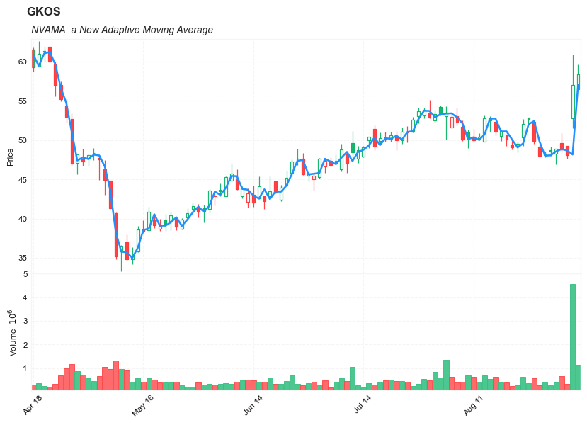
ticker = 'GKOS'
dfs[ticker].tail(5)
| Open | High | Low | Close | Volume | Dividends | Stock Splits | |
|---|---|---|---|---|---|---|---|
| Date | |||||||
| 2022-09-01 | 48.209999 | 48.919998 | 46.900002 | 48.840000 | 372500 | 0 | 0 |
| 2022-09-02 | 49.590000 | 50.900002 | 48.419998 | 48.830002 | 650900 | 0 | 0 |
| 2022-09-06 | 49.200001 | 49.200001 | 47.630001 | 48.099998 | 334400 | 0 | 0 |
| 2022-09-07 | 52.759998 | 60.919998 | 51.490002 | 57.009998 | 4560500 | 0 | 0 |
| 2022-09-08 | 56.439999 | 59.599998 | 56.439999 | 58.380001 | 1106900 | 0 | 0 |
Define NVAMA calculation function
//@version=2
study("VAMA",overlay=true)
length = input(14)
//----
c = sma(close,length)
o = sma(open,length)
h = sma(high,length)
l = sma(low,length)
lv = abs(c-o)/(h - l)
//----
ma = lv*close+(1-lv)*nz(ma[1],close)
plot(ma,color=#FF0000,transp=0)
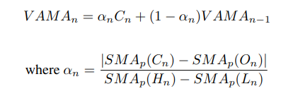
def cal_nvama(ohlc: pd.DataFrame, period: int = 14) -> pd.Series:
        """
        A New Adaptive Moving Average: VAMA
        :period: Specifies the number of periods used for VAMA calculation

        based on: https://mpra.ub.uni-muenchen.de/94323/1/MPRA_paper_94323.pdf

        """
        ohlc = ohlc.copy(deep=True)
        ohlc.columns = [col_name.lower() for col_name in ohlc.columns]
        c = ohlc.close.rolling(period).mean()
        o = ohlc.open.rolling(period).mean()
        h = ohlc.high.rolling(period).mean()
        l = ohlc.low.rolling(period).mean()

        lv = abs(c - o)/(h - l)
        ma = lv*ohlc.close + (1 - lv)*ohlc.close.shift(1)


        return pd.Series(ma, index=ohlc.index, name=f"NVAMA{period}")
Calculate NVAMA
df = dfs[ticker][['Open', 'High', 'Low', 'Close', 'Volume']]
df = df.round(2)
df_ta = cal_nvama(df, period = 14)
df = df.merge(df_ta, left_index = True, right_index = True, how='inner' )

del df_ta
gc.collect()
101
display(df.head(5))
display(df.tail(5))
| Open | High | Low | Close | Volume | NVAMA14 | |
|---|---|---|---|---|---|---|
| Date | ||||||
| 2015-06-25 | 29.11 | 31.95 | 28.00 | 31.22 | 7554700 | NaN |
| 2015-06-26 | 30.39 | 30.39 | 27.51 | 28.00 | 1116500 | NaN |
| 2015-06-29 | 27.70 | 28.48 | 27.51 | 28.00 | 386900 | NaN |
| 2015-06-30 | 27.39 | 29.89 | 27.39 | 28.98 | 223900 | NaN |
| 2015-07-01 | 28.83 | 29.00 | 27.87 | 28.00 | 150000 | NaN |
| Open | High | Low | Close | Volume | NVAMA14 | |
|---|---|---|---|---|---|---|
| Date | ||||||
| 2022-09-01 | 48.21 | 48.92 | 46.90 | 48.84 | 372500 | 48.553668 |
| 2022-09-02 | 49.59 | 50.90 | 48.42 | 48.83 | 650900 | 48.838361 |
| 2022-09-06 | 49.20 | 49.20 | 47.63 | 48.10 | 334400 | 48.667913 |
| 2022-09-07 | 52.76 | 60.92 | 51.49 | 57.01 | 4560500 | 48.147812 |
| 2022-09-08 | 56.44 | 59.60 | 56.44 | 58.38 | 1106900 | 57.072998 |
#https://github.com/matplotlib/mplfinance
#this package help visualize financial data
import mplfinance as mpf
import matplotlib.colors as mcolors

# all_colors = list(mcolors.CSS4_COLORS.keys())#"CSS Colors"
all_colors = list(mcolors.TABLEAU_COLORS.keys()) # "Tableau Palette",
# all_colors = list(mcolors.BASE_COLORS.keys()) #"Base Colors",


#https://github.com/matplotlib/mplfinance/issues/181#issuecomment-667252575
#list of colors: https://matplotlib.org/stable/gallery/color/named_colors.html
#https://github.com/matplotlib/mplfinance/blob/master/examples/styles.ipynb

def plot_3panels(main_data, add_data=None, mid_panel=None, chart_type='candle', names=None,
                  figratio=(14,9)):


    style = mpf.make_mpf_style(base_mpf_style='yahoo',  #charles
                               base_mpl_style = 'seaborn-whitegrid',
#                                marketcolors=mpf.make_marketcolors(up="r", down="#0000CC",inherit=True),
                               gridcolor="whitesmoke",
                               gridstyle="--", #or None, or - for solid
                               gridaxis="both",
                               edgecolor = 'whitesmoke',
                               facecolor = 'white', #background color within the graph edge
                               figcolor = 'white', #background color outside of the graph edge
                               y_on_right = False,
                               rc =  {'legend.fontsize': 'small',#or number
                                      #'figure.figsize': (14, 9),
                                     'axes.labelsize': 'small',
                                     'axes.titlesize':'small',
                                     'xtick.labelsize':'small',#'x-small', 'small','medium','large'
                                     'ytick.labelsize':'small'
                                     },
                              )

    if (chart_type is None) or (chart_type not in ['ohlc', 'line', 'candle', 'hollow_and_filled']):
        chart_type = 'candle'
    len_dict = {'candle':2, 'ohlc':3, 'line':1, 'hollow_and_filled':2}

    kwargs = dict(type=chart_type, figratio=figratio, volume=True, volume_panel=1,
                  panel_ratios=(4,2), tight_layout=True, style=style, returnfig=True)

    if names is None:
        names = {'main_title': '', 'sub_tile': ''}


    added_plots = {

        'NVAMA14': mpf.make_addplot(add_data['NVAMA14'], panel=0, color='dodgerblue', secondary_y=False),
#         'AO-SIGNAL': mpf.make_addplot(mid_panel['AO']-mid_panel['SIGNAL'], type='bar',width=0.7,panel=1, color="pink",alpha=0.65,secondary_y=False),
    }


    fig, axes = mpf.plot(main_data,  **kwargs,
                         addplot=list(added_plots.values()),
                        )
    # add a new suptitle
    fig.suptitle(names['main_title'], y=1.05, fontsize=12, x=0.128)

    axes[0].set_title(names['sub_tile'], fontsize=10, style='italic',  loc='left')


    #set legend

#     axes[0].legend([None]*6)
#     handles = axes[0].get_legend().legendHandles
#     print(handles)
#     axes[0].legend(handles=handles[4:],labels=['MAMA', 'FAMA'])
    #axes[2].set_title('AO', fontsize=10, style='italic',  loc='left')
#     axes[0].set_ylabel('MAMA')


#     axes[0].set_ylabel(names['y_tiles'][0])
    return fig, axes
start = -100
end = df.shape[0]

names = {'main_title': f'{ticker}',
         'sub_tile': 'NVAMA: a New Adaptive Moving Average'}


aa_, bb_ = plot_3panels(df.iloc[start:end][['Open', 'High', 'Low', 'Close', 'Volume']],
             df.iloc[start:end][[ 'NVAMA14']],
             None,
             chart_type='hollow_and_filled',
                     names = names,
                    )