Aroon
References
Definition
The Aroon indicators
measure the number of periods since price recorded an x-day high or low. AroonUp is based on price highs, while Aroon-Down is based on price lows. The Aroon indicators are shown in percentage terms and fluctuate between 0 and 100. View on a particular stock is bullish Aroon-Up is above 50 and Aroon-Down is below 50. This indicates a greater propensity for new x-day highs than lows. The converse is true for a downtrend. The view on a stock is bearish when Aroon-Up is below 50 and Aroon-Down is above 50. The calculation of the Aroon indicator is mentioned in the link in the bibliography.
Load basic packages
import pandas as pd
import numpy as np
import os
import gc
import copy
from pathlib import Path
from datetime import datetime, timedelta, time, date
#this package is to download equity price data from yahoo finance
#the source code of this package can be found here: https://github.com/ranaroussi/yfinance/blob/main
import yfinance as yf
pd.options.display.max_rows = 100
pd.options.display.max_columns = 100

import warnings
warnings.filterwarnings("ignore")

import pytorch_lightning as pl
random_seed=1234
pl.seed_everything(random_seed)
Global seed set to 1234


1234
#S&P 500 (^GSPC),  Dow Jones Industrial Average (^DJI), NASDAQ Composite (^IXIC)
#Russell 2000 (^RUT), Crude Oil Nov 21 (CL=F), Gold Dec 21 (GC=F)
#Treasury Yield 10 Years (^TNX)

#benchmark_tickers = ['^GSPC', '^DJI', '^IXIC', '^RUT',  'CL=F', 'GC=F', '^TNX']

benchmark_tickers = ['^GSPC']
tickers = benchmark_tickers + ['GSK', 'NVO', 'PFE']
#https://github.com/ranaroussi/yfinance/blob/main/yfinance/base.py
#     def history(self, period="1mo", interval="1d",
#                 start=None, end=None, prepost=False, actions=True,
#                 auto_adjust=True, back_adjust=False,
#                 proxy=None, rounding=False, tz=None, timeout=None, **kwargs):

dfs = {}

for ticker in tickers:
    cur_data = yf.Ticker(ticker)
    hist = cur_data.history(period="max", start='2000-01-01')
    print(datetime.now(), ticker, hist.shape, hist.index.min(), hist.index.max())
    dfs[ticker] = hist
2022-09-07 09:41:17.067982 ^GSPC (5707, 7) 1999-12-31 00:00:00 2022-09-06 00:00:00
2022-09-07 09:41:17.398588 GSK (5707, 7) 1999-12-31 00:00:00 2022-09-06 00:00:00
2022-09-07 09:41:17.789028 NVO (5707, 7) 1999-12-31 00:00:00 2022-09-06 00:00:00
2022-09-07 09:41:18.193807 PFE (5707, 7) 1999-12-31 00:00:00 2022-09-06 00:00:00
ticker = 'GSK'
dfs[ticker].tail(5)
| Open | High | Low | Close | Volume | Dividends | Stock Splits | |
|---|---|---|---|---|---|---|---|
| Date | |||||||
| 2022-08-30 | 33.230000 | 33.290001 | 32.919998 | 32.959999 | 3994500 | 0.0 | 0.0 |
| 2022-08-31 | 32.790001 | 32.880001 | 32.459999 | 32.480000 | 4291800 | 0.0 | 0.0 |
| 2022-09-01 | 31.830000 | 31.990000 | 31.610001 | 31.690001 | 12390900 | 0.0 | 0.0 |
| 2022-09-02 | 31.600000 | 31.969999 | 31.469999 | 31.850000 | 8152600 | 0.0 | 0.0 |
| 2022-09-06 | 31.650000 | 31.760000 | 31.370001 | 31.469999 | 5613900 | 0.0 | 0.0 |
Define Aroon calculation function
def cal_aroon(ohlc: pd.DataFrame, period: int = 10) -> pd.DataFrame:
    """
    The Aroon indicators measure the number of periods since price recorded an x-day high or low. AroonUp is based on price highs, while Aroon-Down is based on price lows. The Aroon indicators are shown
    in percentage terms and fluctuate between 0 and 100. View on a particular stock is bullish Aroon-Up
    is above 50 and Aroon-Down is below 50. This indicates a greater propensity for new x-day highs than
    lows. The converse is true for a downtrend. The view on a stock is bearish when Aroon-Up is below
    50 and Aroon-Down is above 50. The calculation of the Aroon indicator is mentioned in the link in
    the bibliography.

    the ohlc datafrome is sorted by 'Date' ascending

    Note the following calculation is wrong in that if there are more than 1 max in the rolling period,
        it will get the first (i.e. the earlies in date) max instead of most recent (i.e. the last) max
        periods = 10
        aroon_up = df['High'].rolling(periods+1).apply(lambda x: x.argmax(), raw=True) / periods * 100
        aroon_down = df['Low'].rolling(periods+1).apply(lambda x: x.argmin(), raw=True) / periods * 100
    """
    ohlc = ohlc.copy()
    ohlc.columns = [c.lower() for c in ohlc.columns]

    high = ohlc["high"]
    low = ohlc["low"]

    hh_loc = high.rolling(period + 1).apply(lambda x: np.argmax(x[::-1]), raw=True)
    ll_loc = low.rolling(period + 1).apply(lambda x: np.argmin(x[::-1]), raw=True)
    aroon_up = 100*(1 - hh_loc/period)
    aroon_down = 100*(1 - ll_loc/period)
    aroon = aroon_up - aroon_down

    return pd.DataFrame(data={'AROON_UP': aroon_up,
                              'AROON_DOWN': aroon_down,
                              'AROON': aroon,
                             },
                        index = ohlc.index)
Calculate AROON
df = dfs[ticker][['Open', 'High', 'Low', 'Close', 'Volume']]
df = df.round(2)
help(cal_aroon)
Help on function cal_aroon in module __main__:

cal_aroon(ohlc: pandas.core.frame.DataFrame, period: int = 10) -> pandas.core.frame.DataFrame
    The Aroon indicators measure the number of periods since price recorded an x-day high or low. AroonUp is based on price highs, while Aroon-Down is based on price lows. The Aroon indicators are shown
    in percentage terms and fluctuate between 0 and 100. View on a particular stock is bullish Aroon-Up
    is above 50 and Aroon-Down is below 50. This indicates a greater propensity for new x-day highs than
    lows. The converse is true for a downtrend. The view on a stock is bearish when Aroon-Up is below
    50 and Aroon-Down is above 50. The calculation of the Aroon indicator is mentioned in the link in
    the bibliography.

    the ohlc datafrome is sorted by 'Date' ascending

    Note the following calculation is wrong in that if there are more than 1 max in the rolling period,
        it will get the first (i.e. the earlies in date) max instead of most recent (i.e. the last) max
        periods = 10
        aroon_up = df['High'].rolling(periods+1).apply(lambda x: x.argmax(), raw=True) / periods * 100
        aroon_down = df['Low'].rolling(periods+1).apply(lambda x: x.argmin(), raw=True) / periods * 100
df_ta = cal_aroon(df, period = 14)
df = df.merge(df_ta, left_index = True, right_index = True, how='inner' )

del df_ta
gc.collect()
11055
from core.finta import TA
help(TA.BBANDS)
Help on function BBANDS in module core.finta:

BBANDS(ohlc: pandas.core.frame.DataFrame, period: int = 20, MA: pandas.core.series.Series = None, column: str = 'close', std_multiplier: float = 2) -> pandas.core.frame.DataFrame
    Developed by John Bollinger, Bollinger Bands® are volatility bands placed above and below a moving average.
    Volatility is based on the standard deviation, which changes as volatility increases and decreases.
    The bands automatically widen when volatility increases and narrow when volatility decreases.

    This method allows input of some other form of moving average like EMA or KAMA around which BBAND will be formed.
    Pass desired moving average as <MA> argument. For example BBANDS(MA=TA.KAMA(20)).
df_ta = TA.BBANDS(df,  period = 20, column="close", std_multiplier=1.95)
df = df.merge(df_ta, left_index = True, right_index = True, how='inner' )

del df_ta
gc.collect()
63
display(df.head(5))
display(df.tail(5))
| Open | High | Low | Close | Volume | AROON_UP | AROON_DOWN | AROON | BB_UPPER | BB_MIDDLE | BB_LOWER | |
|---|---|---|---|---|---|---|---|---|---|---|---|
| Date | |||||||||||
| 1999-12-31 | 19.60 | 19.67 | 19.52 | 19.56 | 139400 | NaN | NaN | NaN | NaN | NaN | NaN |
| 2000-01-03 | 19.58 | 19.71 | 19.25 | 19.45 | 556100 | NaN | NaN | NaN | NaN | NaN | NaN |
| 2000-01-04 | 19.45 | 19.45 | 18.90 | 18.95 | 367200 | NaN | NaN | NaN | NaN | NaN | NaN |
| 2000-01-05 | 19.21 | 19.58 | 19.08 | 19.58 | 481700 | NaN | NaN | NaN | NaN | NaN | NaN |
| 2000-01-06 | 19.38 | 19.43 | 18.90 | 19.30 | 853800 | NaN | NaN | NaN | NaN | NaN | NaN |
| Open | High | Low | Close | Volume | AROON_UP | AROON_DOWN | AROON | BB_UPPER | BB_MIDDLE | BB_LOWER | |
|---|---|---|---|---|---|---|---|---|---|---|---|
| Date | |||||||||||
| 2022-08-30 | 33.23 | 33.29 | 32.92 | 32.96 | 3994500 | 0.000000 | 100.0 | -100.000000 | 41.099946 | 35.7605 | 30.421054 |
| 2022-08-31 | 32.79 | 32.88 | 32.46 | 32.48 | 4291800 | 7.142857 | 100.0 | -92.857143 | 40.446679 | 35.3665 | 30.286321 |
| 2022-09-01 | 31.83 | 31.99 | 31.61 | 31.69 | 12390900 | 0.000000 | 100.0 | -100.000000 | 39.764640 | 34.9440 | 30.123360 |
| 2022-09-02 | 31.60 | 31.97 | 31.47 | 31.85 | 8152600 | 7.142857 | 100.0 | -92.857143 | 38.904860 | 34.5310 | 30.157140 |
| 2022-09-06 | 31.65 | 31.76 | 31.37 | 31.47 | 5613900 | 0.000000 | 100.0 | -100.000000 | 37.934857 | 34.1115 | 30.288143 |
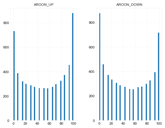
df[['AROON_UP', 'AROON_DOWN']].hist(bins=50)
array([[<AxesSubplot:title={'center':'AROON_UP'}>,
        <AxesSubplot:title={'center':'AROON_DOWN'}>]], dtype=object)
#https://github.com/matplotlib/mplfinance
#this package help visualize financial data
import mplfinance as mpf
import matplotlib.colors as mcolors

# all_colors = list(mcolors.CSS4_COLORS.keys())#"CSS Colors"
# all_colors = list(mcolors.TABLEAU_COLORS.keys()) # "Tableau Palette",
# all_colors = list(mcolors.BASE_COLORS.keys()) #"Base Colors",
all_colors = ['dodgerblue', 'firebrick','limegreen','skyblue','lightgreen',  'navy','yellow','plum',  'yellowgreen']
#https://github.com/matplotlib/mplfinance/issues/181#issuecomment-667252575
#list of colors: https://matplotlib.org/stable/gallery/color/named_colors.html
#https://github.com/matplotlib/mplfinance/blob/master/examples/styles.ipynb

def make_3panels2(main_data, add_data, mid_panel=None, chart_type='candle', names=None, figratio=(14,9)):
    """
    main chart type: default is candle. alternatives: ohlc, line

    example:
    start = 200

    names = {'main_title': 'MAMA: MESA Adaptive Moving Average',
             'sub_tile': 'S&P 500 (^GSPC)', 'y_tiles': ['price', 'Volume [$10^{6}$]']}


    make_candle(df.iloc[-start:, :5], df.iloc[-start:][['MAMA', 'FAMA']], names = names)

    """

    style = mpf.make_mpf_style(base_mpf_style='yahoo',  #charles
                               base_mpl_style = 'seaborn-whitegrid',
#                                marketcolors=mpf.make_marketcolors(up="r", down="#0000CC",inherit=True),
                               gridcolor="whitesmoke",
                               gridstyle="--", #or None, or - for solid
                               gridaxis="both",
                               edgecolor = 'whitesmoke',
                               facecolor = 'white', #background color within the graph edge
                               figcolor = 'white', #background color outside of the graph edge
                               y_on_right = False,
                               rc =  {'legend.fontsize': 'small',#or number
                                      #'figure.figsize': (14, 9),
                                     'axes.labelsize': 'small',
                                     'axes.titlesize':'small',
                                     'xtick.labelsize':'small',#'x-small', 'small','medium','large'
                                     'ytick.labelsize':'small'
                                     },
                              )

    if (chart_type is None) or (chart_type not in ['ohlc', 'line', 'candle', 'hollow_and_filled']):
        chart_type = 'candle'
    len_dict = {'candle':2, 'ohlc':3, 'line':1, 'hollow_and_filled':2}

    kwargs = dict(type=chart_type, figratio=figratio, volume=False, volume_panel=1,
                  panel_ratios=(4,2), tight_layout=True, style=style, returnfig=True)

    if names is None:
        names = {'main_title': '', 'sub_tile': ''}


    added_plots = { }
    for name_, data_ in add_data.iteritems():
        added_plots[name_] = mpf.make_addplot(data_, panel=0, width=1, secondary_y=False)

    fb_bbands_ = dict(y1=add_data.iloc[:, 0].values,
                      y2=add_data.iloc[:, 1].values,color="lightskyblue",alpha=0.1,interpolate=True)
    fb_bbands_['panel'] = 0


    fb_bbands= [fb_bbands_]


    if mid_panel is not None:
        i = 0
        for name_, data_ in mid_panel.iteritems():
            added_plots[name_] = mpf.make_addplot(data_, panel=1, color=all_colors[i])
            i = i + 1
        fb_bbands2_ = dict(y1=np.zeros(mid_panel.shape[0]),
                      y2=0.8+np.zeros(mid_panel.shape[0]),color="lightskyblue",alpha=0.1,interpolate=True)
        fb_bbands2_['panel'] = 1
        fb_bbands.append(fb_bbands2_)


    fig, axes = mpf.plot(main_data,  **kwargs,
                         addplot=list(added_plots.values()),
                         fill_between=fb_bbands)
    # add a new suptitle
    fig.suptitle(names['main_title'], y=1.05, fontsize=12, x=0.1285)

#     axes[0].legend([None]*5)
#     handles = axes[0].get_legend().legendHandles
#     axes[0].legend(handles=handles[2:],labels=list(added_plots.keys()))
    axes[0].set_title(names['sub_tile'], fontsize=10, style='italic',  loc='left')


#     axes[0].set_ylabel(names['y_tiles'][0])
#     axes[2].set_ylabel(names['y_tiles'][1])
    return fig, axes
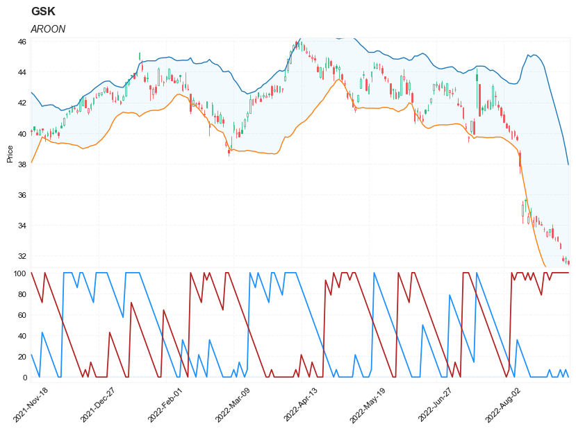
start = -200
end = df.shape[0]

names = {'main_title': f'{ticker}',
         'sub_tile': 'AROON'}


aa_, bb_ = make_3panels2(df.iloc[start:end][['Open', 'High', 'Low', 'Close', 'Volume']],
            df.iloc[start:end][['BB_UPPER', 'BB_LOWER' ]],
            df.iloc[start:end][['AROON_UP', 'AROON_DOWN']],
             chart_type='hollow_and_filled',names = names)
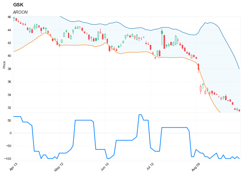
start = -100
end = df.shape[0]

names = {'main_title': f'{ticker}',
         'sub_tile': 'AROON'}


aa_, bb_ = make_3panels2(df.iloc[start:end][['Open', 'High', 'Low', 'Close', 'Volume']],
            df.iloc[start:end][['BB_UPPER', 'BB_LOWER' ]],
            df.iloc[start:end][['AROON',]],
             chart_type='hollow_and_filled',names = names)