Measuring Overbought And Oversold: Greed And Fear Index (GFI)
█ OVERVIEW
In his article in Oct 2022 issue of Technical Analysis of Stocks and Commodities, “Measuring Overbought And Oversold: Greed And Fear Index” author Howard Wang describes the construction of greed and fear index (GFI).
In simple terms, the GFI helps to detect selling and buying earlier in the trend rather than later in the trend:
- A high GFI implies that there is overheated buying sentiment and that traders may have overbought. A high GFI may be a good time to sell ahead of the crowd and ahead of a possible reversal.
- A very low GFI may indicate a good time to buy in advance of the crowd.
█ CALCULATION
As with the BRSI, calculation of the GFI is according to the breakout candlestick. “BOK” stands for “breakout candlestick” and is formed from five original candles:
- BOKH (BOK candles high) (BOKH is the 5 highest candles)
- BOKL (BOK candles low) (BOKL is the 5 lowest candles)
- BOKC (BOK candles close) (BOKC is the 5 last closes)
- BOKO (BOK candles open) (BOKO is the 5 last opens)
The formula for the GFI is: GFI = B⁄A
- B = Mean of (BOKC−BOKO) for 5 periods
- A = Mean of (BOKH−BOKL) for 5 periods
█ EXPLANATION
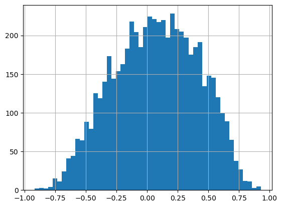
GFI ranges between +1 and −1:
- If GFI is close to +1, it indicates there is overheated buying sentiment and traders may have overbought by this point. This may be a good time to sell in advance of the crowd, in order to sell close to a top.
- If GFI is close to −1, it indicates that stop losses are being hit, indicating selling, and the market may be reaching an oversold condition. This may be a good time to buy in advance of the crowd (that is, buy the dip).
- If GFI = 0, it indicates we are at an inflection point, which means a change may be about to occur in the current buy sell activity.
Load basic packages
import pandas as pd
import numpy as np
import os
import gc
import copy
from pathlib import Path
from datetime import datetime, timedelta, time, date
#this package is to download equity price data from yahoo finance
#the source code of this package can be found here: https://github.com/ranaroussi/yfinance/blob/main
import yfinance as yf
pd.options.display.max_rows = 100
pd.options.display.max_columns = 100

import warnings
warnings.filterwarnings("ignore")

import pytorch_lightning as pl
random_seed=1234
pl.seed_everything(random_seed)
1234
Download data
#S&P 500 (^GSPC),  Dow Jones Industrial Average (^DJI), NASDAQ Composite (^IXIC)
#Russell 2000 (^RUT), Crude Oil Nov 21 (CL=F), Gold Dec 21 (GC=F)
#Treasury Yield 10 Years (^TNX)
#CBOE Volatility Index (^VIX) Chicago Options - Chicago Options Delayed Price. Currency in USD

#benchmark_tickers = ['^GSPC', '^DJI', '^IXIC', '^RUT',  'CL=F', 'GC=F', '^TNX']

benchmark_tickers = ['^GSPC', '^VIX']
tickers = benchmark_tickers + ['GSK', 'BST', 'PFE', 'AZN', 'BSX', 'NUVA', 'MDT']
#https://github.com/ranaroussi/yfinance/blob/main/yfinance/base.py
#     def history(self, period="1mo", interval="1d",
#                 start=None, end=None, prepost=False, actions=True,
#                 auto_adjust=True, back_adjust=False,
#                 proxy=None, rounding=False, tz=None, timeout=None, **kwargs):

dfs = {}

for ticker in tickers:
    cur_data = yf.Ticker(ticker)
    hist = cur_data.history(period="max", start='2000-01-01')
    print(f"{datetime.now()}\t {ticker}\t {hist.shape}\t {hist.index.min()}\t {hist.index.max()}")
    dfs[ticker] = hist
2023-03-08 13:50:01.144419	 ^GSPC	 (5831, 7)	 2000-01-03 00:00:00-05:00	 2023-03-07 00:00:00-05:00
2023-03-08 13:50:02.185163	 ^VIX	 (5832, 7)	 2000-01-03 00:00:00-05:00	 2023-03-08 00:00:00-05:00
2023-03-08 13:50:03.568624	 GSK	 (5831, 7)	 2000-01-03 00:00:00-05:00	 2023-03-07 00:00:00-05:00
2023-03-08 13:50:04.503930	 BST	 (2102, 7)	 2014-10-29 00:00:00-04:00	 2023-03-07 00:00:00-05:00
2023-03-08 13:50:05.765909	 PFE	 (5831, 7)	 2000-01-03 00:00:00-05:00	 2023-03-07 00:00:00-05:00
2023-03-08 13:50:07.133366	 AZN	 (5831, 7)	 2000-01-03 00:00:00-05:00	 2023-03-07 00:00:00-05:00
2023-03-08 13:50:08.237812	 BSX	 (5831, 7)	 2000-01-03 00:00:00-05:00	 2023-03-07 00:00:00-05:00
2023-03-08 13:50:09.634396	 NUVA	 (4736, 7)	 2004-05-13 00:00:00-04:00	 2023-03-07 00:00:00-05:00
2023-03-08 13:50:11.039413	 MDT	 (5831, 7)	 2000-01-03 00:00:00-05:00	 2023-03-07 00:00:00-05:00
ticker = '^GSPC'
dfs[ticker].tail(5)
| Open | High | Low | Close | Volume | Dividends | Stock Splits | |
|---|---|---|---|---|---|---|---|
| Date | |||||||
| 2023-03-01 00:00:00-05:00 | 3963.340088 | 3971.729980 | 3939.050049 | 3951.389893 | 4249480000 | 0.0 | 0.0 |
| 2023-03-02 00:00:00-05:00 | 3938.679932 | 3990.840088 | 3928.159912 | 3981.350098 | 4244900000 | 0.0 | 0.0 |
| 2023-03-03 00:00:00-05:00 | 3998.020020 | 4048.290039 | 3995.169922 | 4045.639893 | 4084730000 | 0.0 | 0.0 |
| 2023-03-06 00:00:00-05:00 | 4055.149902 | 4078.489990 | 4044.610107 | 4048.419922 | 4000870000 | 0.0 | 0.0 |
| 2023-03-07 00:00:00-05:00 | 4048.260010 | 4050.000000 | 3980.310059 | 3986.370117 | 3922500000 | 0.0 | 0.0 |
Define Greed And Fear Index (GFI) calculation function
import sys
sys.path.append(r"/kaggle/input/technical-indicators-core")

#from core.finta import TA
from finta import TA
df = dfs[ticker][['Open', 'High', 'Low', 'Close', 'Volume']]
df = df.round(2)
def cal_gfi(ohlc: pd.DataFrame,
                  period: int = 5,
                 ) -> pd.Series:
    """
    // TASC Oct 2022: Measuring Overbought And Oversold: Greed And Fear Index by Howard Wang

    """

    ohlc = ohlc.copy(deep=True)
    ohlc.columns = [c.lower() for c in ohlc.columns]

    #step 1: get the breakout candlesticks

    break_high = ohlc["high"].rolling(window=2).max()
    break_low = ohlc["low"].rolling(window=2).min()
    two_signs = np.sign(ohlc["close"]-ohlc["open"]).rolling(window=2).apply(np.prod)
    break_open = ohlc["close"].shift(1)
    break_open[two_signs>0] = (ohlc["open"].shift(1))[two_signs>0]
    break_close = ohlc["close"]

    df_break = pd.concat([break_open,break_high, break_low,  break_close], axis=1)
    df_break.columns = ['open', 'high', 'low', 'close']

    #step 2: calculate the GFI

    B = (df_break["close"] - df_break["open"]).rolling(window=period).mean()
    A = (df_break["high"] - df_break["low"]).rolling(window=period).mean()


    return pd.Series(B/A, index=ohlc.index, name=f"GFI{period}")
Calculate Greed And Fear Index (GFI)
df['GFI']=cal_gfi(df)
df['RSI']=TA.RSI(df, period = 14, column="close")
df['EMA50']=TA.EMA(df, period = 50, column="close")
df['EMA200']=TA.EMA(df, period = 200, column="close")
display(df.head(5))
display(df.tail(5))
| Open | High | Low | Close | Volume | GFI | RSI | EMA50 | EMA200 | |
|---|---|---|---|---|---|---|---|---|---|
| Date | |||||||||
| 2000-01-03 00:00:00-05:00 | 1469.25 | 1478.00 | 1438.36 | 1455.22 | 931800000 | NaN | NaN | 1455.220000 | 1455.220000 |
| 2000-01-04 00:00:00-05:00 | 1455.22 | 1455.22 | 1397.43 | 1399.42 | 1009000000 | NaN | 0.000000 | 1426.762000 | 1427.180500 |
| 2000-01-05 00:00:00-05:00 | 1399.42 | 1413.27 | 1377.68 | 1402.11 | 1085500000 | NaN | 4.935392 | 1418.213826 | 1418.739960 |
| 2000-01-06 00:00:00-05:00 | 1402.11 | 1411.90 | 1392.10 | 1403.45 | 1092300000 | NaN | 7.387438 | 1414.298520 | 1414.859942 |
| 2000-01-07 00:00:00-05:00 | 1403.45 | 1441.47 | 1400.73 | 1441.47 | 1225200000 | NaN | 48.207241 | 1420.176074 | 1420.288924 |
| Open | High | Low | Close | Volume | GFI | RSI | EMA50 | EMA200 | |
|---|---|---|---|---|---|---|---|---|---|
| Date | |||||||||
| 2023-03-01 00:00:00-05:00 | 3963.34 | 3971.73 | 3939.05 | 3951.39 | 4249480000 | -0.235848 | 40.292240 | 4004.483349 | 4007.101141 |
| 2023-03-02 00:00:00-05:00 | 3938.68 | 3990.84 | 3928.16 | 3981.35 | 4244900000 | -0.174370 | 44.519159 | 4003.576159 | 4006.844911 |
| 2023-03-03 00:00:00-05:00 | 3998.02 | 4048.29 | 3995.17 | 4045.64 | 4084730000 | 0.268026 | 52.319603 | 4005.225721 | 4007.230932 |
| 2023-03-06 00:00:00-05:00 | 4055.15 | 4078.49 | 4044.61 | 4048.42 | 4000870000 | 0.245390 | 52.629750 | 4006.919615 | 4007.640773 |
| 2023-03-07 00:00:00-05:00 | 4048.26 | 4050.00 | 3980.31 | 3986.37 | 3922500000 | 0.106727 | 45.513517 | 4006.113747 | 4007.429124 |
df['GFI'].hist(bins=50)
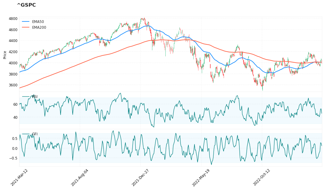
Visualize Greed And Fear Index (GFI)
#from core.visuals import *
from visuals import *
start = -500
end = df.shape[0]
df_sub = df.iloc[start:end]
# df_sub = df[(df.index<='2019-04-01') & (df.index>='2019-01-24')]
#names = {'main_title': f'{ticker}'}
names = {'main_title': f'{ticker} - Greed And Fear Index (GFI)'}

lines0,  ax_cfg0 = plot_overlay_lines(data = df_sub, overlay_columns = ['EMA50', 'EMA200'])

#lines1, ax_cfg1 = plot_macd(data = df_sub, macd= 'DI_PLUS', macd_signal = 'DI_MINUS', panel =1)

lines1, shadows1, ax_cfg1 = plot_add_lines(data = df_sub, line_columns=['RSI', ],
                                           panel =1, bands = [30, 70])
lines2, shadows2, ax_cfg2 = plot_add_lines(data = df_sub, line_columns=['GFI'],
                                           panel =2, bands = [-0.75, 0.75])
#b_s_ = plot_buy_sell(data=df_sub, buy_column='DMI_BUY_Close', sell_column='DMI_SELL_Close')
lines_ = dict(**lines0, **lines1)
lines_.update(lines2)
#lines_.update(b_s_)

shadows_ =    shadows1 + shadows2


fig_config_ = dict(figratio=(18,9), volume=False, volume_panel=2,panel_ratios=(4,2,2), tight_layout=True, returnfig=True,)

ax_cfg_ = ax_cfg0
ax_cfg_.update(ax_cfg1)
ax_cfg_.update(ax_cfg2)


names = {'main_title': f'{ticker}'}

aa_, bb_ = make_panels(main_data = df_sub[['Open', 'High', 'Low', 'Close', 'Volume']],
                       added_plots = lines_,
                       fill_betweens = shadows_,
                       fig_config = fig_config_,
                       axes_config = ax_cfg_,
                       names = names)
Call the function from finta.py
df_list = []
for ticker, df in dfs.items():
    df = df[['Open', 'High', 'Low', 'Close', 'Volume']].round(2)
    #df['GFI']=cal_gfi(df)
    df['GFI']=TA.GFI(df, period = 5)
    df['RSI']=TA.RSI(df, period = 14, column="close")
    df['EMA50']=TA.EMA(df, period = 50, column="close")
    df['EMA200']=TA.EMA(df, period = 200, column="close")
    df['ticker'] = ticker

    df_list.append(df)
df_all = pd.concat(df_list)
print(df_all.shape)
del df_list
gc.collect()
(47656, 10)


5507
dd = df_all.index
df_all.index = dd.date
df_all.index.name='Date'
df_all.tail(5)
| Open | High | Low | Close | Volume | GFI | RSI | EMA50 | EMA200 | ticker | |
|---|---|---|---|---|---|---|---|---|---|---|
| Date | ||||||||||
| 2023-03-01 | 82.40 | 82.53 | 81.67 | 82.08 | 5249100 | -0.449129 | 44.022248 | 82.552691 | 86.762242 | MDT |
| 2023-03-02 | 81.49 | 82.56 | 81.20 | 82.26 | 4985100 | -0.268898 | 44.950352 | 82.541213 | 86.717444 | MDT |
| 2023-03-03 | 82.79 | 83.63 | 82.44 | 83.41 | 4771600 | -0.007821 | 50.587132 | 82.575283 | 86.684534 | MDT |
| 2023-03-06 | 83.49 | 83.83 | 81.45 | 81.93 | 6845500 | -0.151832 | 44.300301 | 82.549978 | 86.637225 | MDT |
| 2023-03-07 | 82.09 | 82.15 | 79.51 | 79.74 | 6876000 | -0.349321 | 36.977231 | 82.439782 | 86.568596 | MDT |
df_all.to_csv('b_055_1_gfi_tasc202210.csv', index=True)