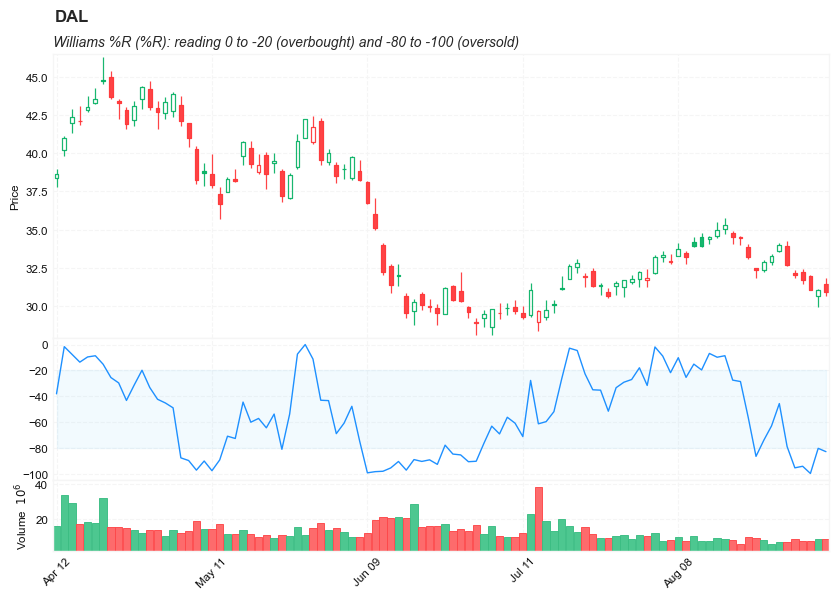
Williams %R (%R)
References
Definition
- Williams %R (%R) is a momentum-based oscillator created by Larry Williams.
- It is used to identify overbought and oversold conditions.
- The %R is based on a comparison between the current close and the highest high for a user defined look back period.
- %R Oscillates between 0 and -100 (note the negative values):
- readings closer to 0 indicating more overbought conditions
- readings closer to -100 indicating oversold.
Calculation
%R = (Highest High - Current Close) / (Highest High - Lowest Low) x -100
- Highest High = Highest High for the user defined look-back period.
- Lowest Low = Lowest Low for the user defined look-back period.
Read the indicator
- Overbought/Oversold
- Overbought conditions (traditionally defined as values between 0 and -20) can indicate either a trend reversal or in many cases, a strengthening of the current trend.
- Oversold conditions (traditionally defined as values between -80 and -100) can indicate either a trend reversal or in many cases, a strengthening of the current trend.
- Momentum Failures
- Momentum failure occur when %R readings reach overbought or oversold conditions for an extended period of time. Upon leaving overbought/oversold territory, %R makes a move back towards the overbought/oversold levels but fails to re-enter the territory.
The traditional 0 to -20 (overbought) and -80 to -100 (oversold) were set by Larry Williams (the creator of the indicator). Depending on multiple factors such as volatility or market news, these standard levels may not be appropriate for every situation. As with most technical analysis tools, the %R is best when used as part of a larger trading system and not necessarily as a stand-alone indicator.
Load basic packages
import pandas as pd
import numpy as np
import os
import gc
import copy
from pathlib import Path
from datetime import datetime, timedelta, time, date
#this package is to download equity price data from yahoo finance
#the source code of this package can be found here: https://github.com/ranaroussi/yfinance/blob/main
import yfinance as yf
pd.options.display.max_rows = 100
pd.options.display.max_columns = 100

import warnings
warnings.filterwarnings("ignore")

import pytorch_lightning as pl
random_seed=1234
pl.seed_everything(random_seed)
Global seed set to 1234


1234
#S&P 500 (^GSPC),  Dow Jones Industrial Average (^DJI), NASDAQ Composite (^IXIC)
#Russell 2000 (^RUT), Crude Oil Nov 21 (CL=F), Gold Dec 21 (GC=F)
#Treasury Yield 10 Years (^TNX)

#benchmark_tickers = ['^GSPC', '^DJI', '^IXIC', '^RUT',  'CL=F', 'GC=F', '^TNX']

benchmark_tickers = ['^GSPC']
tickers = benchmark_tickers + ['GSK', 'NVO', 'PFE', 'DAL']
#https://github.com/ranaroussi/yfinance/blob/main/yfinance/base.py
#     def history(self, period="1mo", interval="1d",
#                 start=None, end=None, prepost=False, actions=True,
#                 auto_adjust=True, back_adjust=False,
#                 proxy=None, rounding=False, tz=None, timeout=None, **kwargs):

dfs = {}

for ticker in tickers:
    cur_data = yf.Ticker(ticker)
    hist = cur_data.history(period="max", start='2000-01-01')
    print(datetime.now(), ticker, hist.shape, hist.index.min(), hist.index.max())
    dfs[ticker] = hist
2022-09-05 18:14:35.339560 ^GSPC (5706, 7) 1999-12-31 00:00:00 2022-09-02 00:00:00
2022-09-05 18:14:35.623208 GSK (5706, 7) 1999-12-31 00:00:00 2022-09-02 00:00:00
2022-09-05 18:14:35.985809 NVO (5706, 7) 1999-12-31 00:00:00 2022-09-02 00:00:00
2022-09-05 18:14:36.355315 PFE (5706, 7) 1999-12-31 00:00:00 2022-09-02 00:00:00
2022-09-05 18:14:36.605538 DAL (3863, 7) 2007-05-03 00:00:00 2022-09-02 00:00:00
ticker = 'DAL'
dfs[ticker].tail(5)
| Open | High | Low | Close | Volume | Dividends | Stock Splits | |
|---|---|---|---|---|---|---|---|
| Date | |||||||
| 2022-08-29 | 32.200001 | 32.349998 | 31.850000 | 32.029999 | 8758400 | 0.0 | 0 |
| 2022-08-30 | 32.250000 | 32.450001 | 31.469999 | 31.719999 | 7506400 | 0.0 | 0 |
| 2022-08-31 | 31.969999 | 32.020000 | 31.059999 | 31.070000 | 7450000 | 0.0 | 0 |
| 2022-09-01 | 30.650000 | 31.139999 | 29.940001 | 31.090000 | 8572700 | 0.0 | 0 |
| 2022-09-02 | 31.440001 | 31.830000 | 30.700001 | 30.940001 | 8626500 | 0.0 | 0 |
Define Williams %R calculation function
#https://github.com/peerchemist/finta/blob/af01fa594995de78f5ada5c336e61cd87c46b151/finta/finta.py


def cal_williams(ohlc: pd.DataFrame, period: int = 14) -> pd.Series:

    """
    Williams %R, or just %R, is a technical analysis oscillator showing the current closing price
    in relation to the high and low of the past N days (for a given N).
    It was developed by a publisher and promoter of trading materials, Larry Williams.
     Its purpose is to tell whether a stock or commodity market is trading near the high or the low, or somewhere in between,
     of its recent trading range.
     The oscillator is on a negative scale, from −100 (lowest) up to 0 (highest).

    """
    ohlc = ohlc.copy(deep=True)
    ohlc.columns = [c.lower() for c in ohlc.columns]

    highest_high = ohlc["high"].rolling(center=False, window=period).max()
    lowest_low = ohlc["low"].rolling(center=False, window=period).min()

    WR = pd.Series(
        (highest_high - ohlc["close"]) / (highest_high - lowest_low),
        name=f"WilliamsR{period}",
    )

    return WR * -100
Calculate Williams %R
df = dfs[ticker][['Open', 'High', 'Low', 'Close', 'Volume']]
df = df.round(2)
cal_williams
<function __main__.cal_williams(ohlc: pandas.core.frame.DataFrame, period: int = 14) -> pandas.core.series.Series>
df_ta = cal_williams(df, period = 14)
df = df.merge(df_ta, left_index = True, right_index = True, how='inner' )

del df_ta
gc.collect()
80
display(df.head(5))
display(df.tail(5))
| Open | High | Low | Close | Volume | WilliamsR14 | |
|---|---|---|---|---|---|---|
| Date | ||||||
| 2007-05-03 | 19.32 | 19.50 | 18.25 | 18.40 | 8052800 | NaN |
| 2007-05-04 | 18.88 | 18.96 | 18.39 | 18.64 | 5437300 | NaN |
| 2007-05-07 | 18.83 | 18.91 | 17.94 | 18.08 | 2646300 | NaN |
| 2007-05-08 | 17.76 | 17.76 | 17.14 | 17.44 | 4166100 | NaN |
| 2007-05-09 | 17.54 | 17.94 | 17.44 | 17.58 | 7541100 | NaN |
| Open | High | Low | Close | Volume | WilliamsR14 | |
|---|---|---|---|---|---|---|
| Date | ||||||
| 2022-08-29 | 32.20 | 32.35 | 31.85 | 32.03 | 8758400 | -95.431472 |
| 2022-08-30 | 32.25 | 32.45 | 31.47 | 31.72 | 7506400 | -94.212963 |
| 2022-08-31 | 31.97 | 32.02 | 31.06 | 31.07 | 7450000 | -99.788584 |
| 2022-09-01 | 30.65 | 31.14 | 29.94 | 31.09 | 8572700 | -80.341880 |
| 2022-09-02 | 31.44 | 31.83 | 30.70 | 30.94 | 8626500 | -82.905983 |
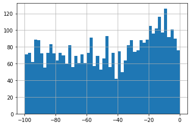
df['WilliamsR14'].hist(bins=50)
<AxesSubplot:>
#https://github.com/matplotlib/mplfinance
#this package help visualize financial data
import mplfinance as mpf
import matplotlib.colors as mcolors

# all_colors = list(mcolors.CSS4_COLORS.keys())#"CSS Colors"
# all_colors = list(mcolors.TABLEAU_COLORS.keys()) # "Tableau Palette",
all_colors = ['dodgerblue', 'firebrick','limegreen','skyblue','lightgreen',  'navy','yellow','plum',  'yellowgreen']
# all_colors = list(mcolors.BASE_COLORS.keys()) #"Base Colors",


#https://github.com/matplotlib/mplfinance/issues/181#issuecomment-667252575
#list of colors: https://matplotlib.org/stable/gallery/color/named_colors.html
#https://github.com/matplotlib/mplfinance/blob/master/examples/styles.ipynb

def make_3panels2(main_data, mid_panel, chart_type='candle', names=None,
                  figratio=(14,9), fill_weights = (0, 0)):
    """
    main chart type: default is candle. alternatives: ohlc, line

    example:
    start = 200

    names = {'main_title': 'MAMA: MESA Adaptive Moving Average',
             'sub_tile': 'S&P 500 (^GSPC)', 'y_tiles': ['price', 'Volume [$10^{6}$]']}


    make_candle(df.iloc[-start:, :5], df.iloc[-start:][['MAMA', 'FAMA']], names = names)

    """

    style = mpf.make_mpf_style(base_mpf_style='yahoo',  #charles
                               base_mpl_style = 'seaborn-whitegrid',
#                                marketcolors=mpf.make_marketcolors(up="r", down="#0000CC",inherit=True),
                               gridcolor="whitesmoke",
                               gridstyle="--", #or None, or - for solid
                               gridaxis="both",
                               edgecolor = 'whitesmoke',
                               facecolor = 'white', #background color within the graph edge
                               figcolor = 'white', #background color outside of the graph edge
                               y_on_right = False,
                               rc =  {'legend.fontsize': 'small',#or number
                                      #'figure.figsize': (14, 9),
                                     'axes.labelsize': 'small',
                                     'axes.titlesize':'small',
                                     'xtick.labelsize':'small',#'x-small', 'small','medium','large'
                                     'ytick.labelsize':'small'
                                     },
                              )

    if (chart_type is None) or (chart_type not in ['ohlc', 'line', 'candle', 'hollow_and_filled']):
        chart_type = 'candle'
    len_dict = {'candle':2, 'ohlc':3, 'line':1, 'hollow_and_filled':2}

    kwargs = dict(type=chart_type, figratio=figratio, volume=True, volume_panel=2,
                  panel_ratios=(4,2,1), tight_layout=True, style=style, returnfig=True)

    if names is None:
        names = {'main_title': '', 'sub_tile': ''}


    added_plots = { }

    fb_bbands2_ = dict(y1=fill_weights[0]*np.ones(mid_panel.shape[0]),
                      y2=fill_weights[1]*np.ones(mid_panel.shape[0]),color="lightskyblue",alpha=0.1,interpolate=True)
    fb_bbands2_['panel'] = 1

    fb_bbands= [fb_bbands2_]


    i = 0
    for name_, data_ in mid_panel.iteritems():
        added_plots[name_] = mpf.make_addplot(data_, panel=1, width=1, color=all_colors[i], secondary_y=False)
        i = i + 1


    fig, axes = mpf.plot(main_data,  **kwargs,
                         addplot=list(added_plots.values()),
                         fill_between=fb_bbands)
    # add a new suptitle
    fig.suptitle(names['main_title'], y=1.05, fontsize=12, x=0.1285)

    axes[0].set_title(names['sub_tile'], fontsize=10, style='italic',  loc='left')
#     axes[2].set_ylabel('WAVEPM10')

#     axes[0].set_ylabel(names['y_tiles'][0])
#     axes[2].set_ylabel(names['y_tiles'][1])
    return fig, axes
start = -100
end = df.shape[0]

names = {'main_title': f'{ticker}',
         'sub_tile': 'Williams %R (%R): reading 0 to -20 (overbought) and -80 to -100 (oversold)'}


aa_, bb_ = make_3panels2(df.iloc[start:end][['Open', 'High', 'Low', 'Close', 'Volume']],
             df.iloc[start:end][['WilliamsR14']],
             chart_type='hollow_and_filled',names = names,
                         fill_weights = (-80, -20))