The Breakout Relative Strength Index (BRSI) by Howard Wang
█ OVERVIEW
In his article in September 2015 issue of Technical Analysis of Stocks and Commodities, “The Breakout Relative Strength Index” author Howard Wang introduced a new indicator that he called “the breakout relative strength index” or BRSI. The BRSI was intended to help traders to determine if a breakout was about to happen as well as the relative strength of the breakout.
█ CALCULATION
There are 2 major steps involved in calculting the BRSI. The first step is to construct the “breakout candlestick” using the original candlestick (i.e. high, low, open, close) data. And the second step is using the “breakout candlestick” along with volume data to calculate the BRSI.
- Step 1: Construct “breakout candlestick”: use 2 days candlestick data (today’s and previous day’s data), the “breakout candlestick”’s high, low, open, close are the following
- use High, Low, Open, Close to denote today’s prices
- use Pre_High, Pre_Low, Pre_Open, Pre_Close to denote previous day’s prices
- use break_High, break_Low, break_Open, break_Close to denote breakout prices
- break_High: max(High, Pre_High), namely the higher of the “High” of the 2 days’ prices
- break_Low: min(Low, Pre_Low),namely the lower of the “Low” of the 2 days data
- break_Open and break_Close:
- If there are two up days or two down days, then the open is the pre-day’s open, and the close is today’s close: If (Close>Open AND Pre_Close>Pre_Open) OR (Close<Open AND Pre_Close<Pre_Open) THEN break_Open=Pre_Open, break_Close=Close
- If there is one up day and one down day, then the open is the pre-day’s close and the close is today’s close: If (Close>Open AND Pre_Close<Pre_Open) OR (Close< Open AND Pre_Close >Pre_Open) THEN break_Open=Pre_Close, break_Close=Close
- Step 2: Calculate BRSI using breakout prices
- High, Low, Open, Close to denote the breakout prices
- Pre_Volume, Volume to denote previous day’s and today’s volume
- breakout price = (High + Low + Open + Close)/4
- breakout volume = (Pre_Volume + Volume)
- breakout strength = (Close - Open)/(High - Low)
- breakout power = breakout price * breakout strength * breakout volume
- if today’s breakout power > previous day’s breakout power then it is Positive power: P = sum of positive power in 14 days
- if today’s breakout power < previous day’s breakout power then it is Negative power: N = sum of absolute value of negative power in 14 days
- breakout ratio = P/N
- BRSI = 100 - (100/1 + breakout ratio)
█ EXPLANATION
BRSI ranges between 0 and 100:
- If BRSI is above 80, it indicates the breakout is strong, the stock is overbought, and the price is likely to go down.
- If BRSI is below 20, it indicates that breakout is weak, the stock is oversold, and the price is likely to go up.
- If BRSI 50, it indicates hold the stock.
Load basic packages
import pandas as pd
import numpy as np
import os
import gc
import copy
from pathlib import Path
from datetime import datetime, timedelta, time, date
#this package is to download equity price data from yahoo finance
#the source code of this package can be found here: https://github.com/ranaroussi/yfinance/blob/main
import yfinance as yf
pd.options.display.max_rows = 100
pd.options.display.max_columns = 100

import warnings
warnings.filterwarnings("ignore")

import pytorch_lightning as pl
random_seed=1234
pl.seed_everything(random_seed)
1234
Download data
#S&P 500 (^GSPC),  Dow Jones Industrial Average (^DJI), NASDAQ Composite (^IXIC)
#Russell 2000 (^RUT), Crude Oil Nov 21 (CL=F), Gold Dec 21 (GC=F)
#Treasury Yield 10 Years (^TNX)
#CBOE Volatility Index (^VIX) Chicago Options - Chicago Options Delayed Price. Currency in USD

#benchmark_tickers = ['^GSPC', '^DJI', '^IXIC', '^RUT',  'CL=F', 'GC=F', '^TNX']

benchmark_tickers = ['^GSPC', '^VIX']
tickers = benchmark_tickers + ['GSK', 'BST', 'PFE', 'AZN', 'BSX', 'NUVA', 'MDT']
#https://github.com/ranaroussi/yfinance/blob/main/yfinance/base.py
#     def history(self, period="1mo", interval="1d",
#                 start=None, end=None, prepost=False, actions=True,
#                 auto_adjust=True, back_adjust=False,
#                 proxy=None, rounding=False, tz=None, timeout=None, **kwargs):

dfs = {}

for ticker in tickers:
    cur_data = yf.Ticker(ticker)
    hist = cur_data.history(period="max", start='2000-01-01')
    print(f"{datetime.now()}\t {ticker}\t {hist.shape}\t {hist.index.min()}\t {hist.index.max()}")
    dfs[ticker] = hist
2023-03-08 12:33:21.731271	 ^GSPC	 (5831, 7)	 2000-01-03 00:00:00-05:00	 2023-03-07 00:00:00-05:00
2023-03-08 12:33:22.023871	 ^VIX	 (5832, 7)	 2000-01-03 00:00:00-05:00	 2023-03-08 00:00:00-05:00
2023-03-08 12:33:22.416429	 GSK	 (5831, 7)	 2000-01-03 00:00:00-05:00	 2023-03-07 00:00:00-05:00
2023-03-08 12:33:22.690798	 BST	 (2102, 7)	 2014-10-29 00:00:00-04:00	 2023-03-07 00:00:00-05:00
2023-03-08 12:33:23.130656	 PFE	 (5831, 7)	 2000-01-03 00:00:00-05:00	 2023-03-07 00:00:00-05:00
2023-03-08 12:33:23.519270	 AZN	 (5831, 7)	 2000-01-03 00:00:00-05:00	 2023-03-07 00:00:00-05:00
2023-03-08 12:33:23.820784	 BSX	 (5831, 7)	 2000-01-03 00:00:00-05:00	 2023-03-07 00:00:00-05:00
2023-03-08 12:33:24.115289	 NUVA	 (4736, 7)	 2004-05-13 00:00:00-04:00	 2023-03-07 00:00:00-05:00
2023-03-08 12:33:24.508971	 MDT	 (5831, 7)	 2000-01-03 00:00:00-05:00	 2023-03-07 00:00:00-05:00
ticker = '^GSPC'
dfs[ticker].tail(5)
| Open | High | Low | Close | Volume | Dividends | Stock Splits | |
|---|---|---|---|---|---|---|---|
| Date | |||||||
| 2023-03-01 00:00:00-05:00 | 3963.340088 | 3971.729980 | 3939.050049 | 3951.389893 | 4249480000 | 0.0 | 0.0 |
| 2023-03-02 00:00:00-05:00 | 3938.679932 | 3990.840088 | 3928.159912 | 3981.350098 | 4244900000 | 0.0 | 0.0 |
| 2023-03-03 00:00:00-05:00 | 3998.020020 | 4048.290039 | 3995.169922 | 4045.639893 | 4084730000 | 0.0 | 0.0 |
| 2023-03-06 00:00:00-05:00 | 4055.149902 | 4078.489990 | 4044.610107 | 4048.419922 | 4000870000 | 0.0 | 0.0 |
| 2023-03-07 00:00:00-05:00 | 4048.260010 | 4050.000000 | 3980.310059 | 3986.370117 | 3922500000 | 0.0 | 0.0 |
Define Breakout Relative Strength Index (BRSI) calculation function
import sys
sys.path.append(r"/kaggle/input/technical-indicators-core")

#from core.finta import TA
from finta import TA
df = dfs[ticker][['Open', 'High', 'Low', 'Close', 'Volume']]
df = df.round(2)
def cal_brsi(ohlcv: pd.DataFrame,
                  period: int = 14,
                 ) -> pd.Series:
    """
    // TASC SEP 2015: The Breakout Relative Strength Index by Howard Wang
    """
    ohlcv = ohlcv.copy(deep=True)
    ohlcv.columns = [c.lower() for c in ohlcv.columns]

    #step 1: get the breakout candlesticks

    break_high = ohlcv["high"].rolling(window=2).max()
    break_low = ohlcv["low"].rolling(window=2).min()
    two_signs = np.sign(ohlcv["close"]-ohlcv["open"]).rolling(window=2).apply(np.prod)
    break_open = ohlcv["close"].shift(1)
    break_open[two_signs>0] = (ohlcv["open"].shift(1))[two_signs>0]
    break_close = ohlcv["close"]

    break_vol = ohlcv["volume"].rolling(window=2).sum()
    df_break = pd.concat([break_open,break_high, break_low,  break_close], axis=1)
    df_break.columns = ['open', 'high', 'low', 'close']

    #step 2: calculate the BRSI

    break_price = df_break[['open', 'high', 'low', 'close']].mean(axis=1)
    break_strength = (df_break["close"] - df_break["open"])/(df_break["high"] - df_break["low"])
    break_power = break_price*break_strength*break_vol

    delta = break_power.diff()

    ## positive gains (up) and negative gains (down) Series
    up, down = delta.copy(), delta.copy()
    up[up < 0] = 0
    down[down > 0] = 0

    _gain = up.rolling(window=period).sum()
    _loss = down.abs().rolling(window=period).sum()

    RS = _gain / _loss

    return pd.Series(100 - (100 / (1 + RS)), index=ohlcv.index, name=f"BRSI{period}")
Calculate Breakout Relative Strength Index (BRSI)
#help(TA.RSI)
df['BRSI']=cal_brsi(df)
df['RSI']=TA.RSI(df, period = 14, column="close")
df['EMA50']=TA.EMA(df, period = 50, column="close")
df['EMA200']=TA.EMA(df, period = 200, column="close")
display(df.head(5))
display(df.tail(5))
| Open | High | Low | Close | Volume | BRSI | RSI | EMA50 | EMA200 | |
|---|---|---|---|---|---|---|---|---|---|
| Date | |||||||||
| 2000-01-03 00:00:00-05:00 | 1469.25 | 1478.00 | 1438.36 | 1455.22 | 931800000 | NaN | NaN | 1455.220000 | 1455.220000 |
| 2000-01-04 00:00:00-05:00 | 1455.22 | 1455.22 | 1397.43 | 1399.42 | 1009000000 | NaN | 0.000000 | 1426.762000 | 1427.180500 |
| 2000-01-05 00:00:00-05:00 | 1399.42 | 1413.27 | 1377.68 | 1402.11 | 1085500000 | NaN | 4.935392 | 1418.213826 | 1418.739960 |
| 2000-01-06 00:00:00-05:00 | 1402.11 | 1411.90 | 1392.10 | 1403.45 | 1092300000 | NaN | 7.387438 | 1414.298520 | 1414.859942 |
| 2000-01-07 00:00:00-05:00 | 1403.45 | 1441.47 | 1400.73 | 1441.47 | 1225200000 | NaN | 48.207241 | 1420.176074 | 1420.288924 |
| Open | High | Low | Close | Volume | BRSI | RSI | EMA50 | EMA200 | |
|---|---|---|---|---|---|---|---|---|---|
| Date | |||||||||
| 2023-03-01 00:00:00-05:00 | 3963.34 | 3971.73 | 3939.05 | 3951.39 | 4249480000 | 50.335227 | 40.292240 | 4004.483349 | 4007.101141 |
| 2023-03-02 00:00:00-05:00 | 3938.68 | 3990.84 | 3928.16 | 3981.35 | 4244900000 | 57.286866 | 44.519159 | 4003.576159 | 4006.844911 |
| 2023-03-03 00:00:00-05:00 | 3998.02 | 4048.29 | 3995.17 | 4045.64 | 4084730000 | 54.623822 | 52.319603 | 4005.225721 | 4007.230932 |
| 2023-03-06 00:00:00-05:00 | 4055.15 | 4078.49 | 4044.61 | 4048.42 | 4000870000 | 45.664820 | 52.629750 | 4006.919615 | 4007.640773 |
| 2023-03-07 00:00:00-05:00 | 4048.26 | 4050.00 | 3980.31 | 3986.37 | 3922500000 | 43.431024 | 45.513517 | 4006.113747 | 4007.429124 |
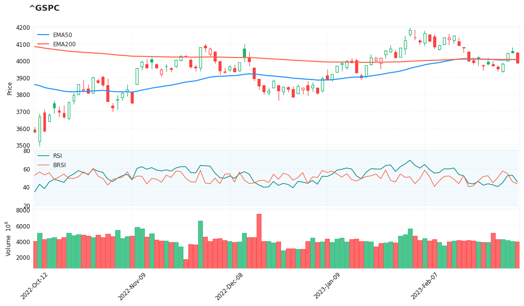
Visualize Breakout Relative Strength Index (BRSI)
#from core.visuals import *
from visuals import *
start = -100
end = df.shape[0]
df_sub = df.iloc[start:end]
# df_sub = df[(df.index<='2019-04-01') & (df.index>='2019-01-24')]
#names = {'main_title': f'{ticker}'}
names = {'main_title': f'{ticker} - Breakout Relative Strength Index (BRSI)'}

lines0,  ax_cfg0 = plot_overlay_lines(data = df_sub, overlay_columns = ['EMA50', 'EMA200'])

#lines1, ax_cfg1 = plot_macd(data = df_sub, macd= 'DI_PLUS', macd_signal = 'DI_MINUS', panel =1)

lines1, shadows1, ax_cfg1 = plot_add_lines(data = df_sub, line_columns=['RSI', 'BRSI'],
                                           panel =1, bands = [20, 80])
#b_s_ = plot_buy_sell(data=df_sub, buy_column='DMI_BUY_Close', sell_column='DMI_SELL_Close')
lines_ = dict(**lines0, **lines1)
#lines_.update(lines2)
#lines_.update(b_s_)

shadows_ =    shadows1


fig_config_ = dict(figratio=(18,9), volume=True, volume_panel=2,panel_ratios=(4,2,2), tight_layout=True, returnfig=True,)

ax_cfg_ = ax_cfg0
ax_cfg_.update(ax_cfg1)
#ax_cfg_.update(ax_cfg2)


names = {'main_title': f'{ticker}'}

aa_, bb_ = make_panels(main_data = df_sub[['Open', 'High', 'Low', 'Close', 'Volume']],
                       added_plots = lines_,
                       fill_betweens = shadows_,
                       fig_config = fig_config_,
                       axes_config = ax_cfg_,
                       names = names)
Call the function from finta.py
#help(TA.BRSI)
df_list = []
for ticker, df in dfs.items():
    df = df[['Open', 'High', 'Low', 'Close', 'Volume']].round(2)

    #df['BRSI']=cal_brsi(df)
    df['BRSI']=TA.BRSI(df, period = 14, )
    df['RSI']=TA.RSI(df, period = 14, column="close")
    df['EMA50']=TA.EMA(df, period = 50, column="close")
    df['EMA200']=TA.EMA(df, period = 200, column="close")
    df['ticker'] = ticker

    df_list.append(df)
df_all = pd.concat(df_list)
print(df_all.shape)
del df_list
gc.collect()
(47656, 10)


7073
dd = df_all.index
df_all.index = dd.date
df_all.index.name='Date'
df_all.tail(5)
| Open | High | Low | Close | Volume | BRSI | RSI | EMA50 | EMA200 | ticker | |
|---|---|---|---|---|---|---|---|---|---|---|
| Date | ||||||||||
| 2023-03-01 | 82.40 | 82.53 | 81.67 | 82.08 | 5249100 | 46.896985 | 44.022248 | 82.552691 | 86.762242 | MDT |
| 2023-03-02 | 81.49 | 82.56 | 81.20 | 82.26 | 4985100 | 56.823645 | 44.950352 | 82.541213 | 86.717444 | MDT |
| 2023-03-03 | 82.79 | 83.63 | 82.44 | 83.41 | 4771600 | 54.858382 | 50.587132 | 82.575283 | 86.684534 | MDT |
| 2023-03-06 | 83.49 | 83.83 | 81.45 | 81.93 | 6845500 | 42.926467 | 44.300301 | 82.549978 | 86.637225 | MDT |
| 2023-03-07 | 82.09 | 82.15 | 79.51 | 79.74 | 6876000 | 46.116515 | 36.977231 | 82.439782 | 86.568596 | MDT |
df_all.to_csv('b_054_1_brsi_tasc201509.csv', index=True)