Commodity Channel Index (CCI)
References
Definition
- The Commodity Channel Index (CCI) is a momentum oscillator
- primarily to identify overbought and oversold levels by measuring an instrument’s variations away from its statistical mean.
- CCI is often used to find reversals and divergences.
Calculation
A typical 20 Period CCI as example:
CCI = (Typical Price - 20 Period SMA of TP) / (.015 x Mean Deviation)
- Typical Price (TP) = (High + Low + Close)/3
- Constant = .015
- The Constant is set at .015 for scaling purposes.
- By including the constant, the majority of CCI values will fall within the 100 to -100 range.
- There are three steps to calculating the Mean Deviation.
- step 1: Subtract the most recent 20 Period Simple Moving from each typical price (TP) for the Period.
- step 2: Sum absolute value of numbers from
step 1. - step 3: Divide the value generated in
step 2by the total number of Periods (20 in this case).
Read the indicator
- The Commodity Channel Index indicator takes a security’s change in price and compares that to its average change in price.
- CCI’s calculation produces positive and negative values that oscillate above and below a Zero Line.
- Typically a value of 100 is identified as overbought and a reading of -100 is identified as being oversold. However,
- Actual overbought and oversold thresholds can vary depending on the financial instrument being traded. For example, a more volatile instrument may have thresholds at 200 and -200.
- when using CCI, overbought and oversold conditions can often be a sign of strength, meaning the current trend may be strengthening and continuing.
Load basic packages
import pandas as pd
import numpy as np
import os
import gc
import copy
from pathlib import Path
from datetime import datetime, timedelta, time, date
#this package is to download equity price data from yahoo finance
#the source code of this package can be found here: https://github.com/ranaroussi/yfinance/blob/main
import yfinance as yf
pd.options.display.max_rows = 100
pd.options.display.max_columns = 100

import warnings
warnings.filterwarnings("ignore")

import pytorch_lightning as pl
random_seed=1234
pl.seed_everything(random_seed)
Global seed set to 1234


1234
#S&P 500 (^GSPC),  Dow Jones Industrial Average (^DJI), NASDAQ Composite (^IXIC)
#Russell 2000 (^RUT), Crude Oil Nov 21 (CL=F), Gold Dec 21 (GC=F)
#Treasury Yield 10 Years (^TNX)

#benchmark_tickers = ['^GSPC', '^DJI', '^IXIC', '^RUT',  'CL=F', 'GC=F', '^TNX']

benchmark_tickers = ['^GSPC']
tickers = benchmark_tickers + ['GSK', 'NVO', 'AROC', 'GKOS']
#https://github.com/ranaroussi/yfinance/blob/main/yfinance/base.py
#     def history(self, period="1mo", interval="1d",
#                 start=None, end=None, prepost=False, actions=True,
#                 auto_adjust=True, back_adjust=False,
#                 proxy=None, rounding=False, tz=None, timeout=None, **kwargs):

dfs = {}

for ticker in tickers:
    cur_data = yf.Ticker(ticker)
    hist = cur_data.history(period="max", start='2000-01-01')
    print(datetime.now(), ticker, hist.shape, hist.index.min(), hist.index.max())
    dfs[ticker] = hist
2022-08-27 18:32:21.399573 ^GSPC (5701, 7) 1999-12-31 00:00:00 2022-08-26 00:00:00
2022-08-27 18:32:21.790691 GSK (5701, 7) 1999-12-31 00:00:00 2022-08-26 00:00:00
2022-08-27 18:32:22.131409 NVO (5701, 7) 1999-12-31 00:00:00 2022-08-26 00:00:00
2022-08-27 18:32:22.407223 AROC (3782, 7) 2007-08-21 00:00:00 2022-08-26 00:00:00
2022-08-27 18:32:22.650068 GKOS (1807, 7) 2015-06-25 00:00:00 2022-08-26 00:00:00
ticker = 'GKOS'
dfs[ticker].tail(5)
| Open | High | Low | Close | Volume | Dividends | Stock Splits | |
|---|---|---|---|---|---|---|---|
| Date | |||||||
| 2022-08-22 | 49.290001 | 50.110001 | 48.810001 | 49.049999 | 243200 | 0 | 0 |
| 2022-08-23 | 49.509998 | 49.759998 | 48.439999 | 49.410000 | 260300 | 0 | 0 |
| 2022-08-24 | 50.290001 | 52.680000 | 49.269001 | 52.000000 | 628200 | 0 | 0 |
| 2022-08-25 | 52.820000 | 52.840000 | 52.040001 | 52.590000 | 349400 | 0 | 0 |
| 2022-08-26 | 52.310001 | 52.580002 | 49.480000 | 49.889999 | 550400 | 0 | 0 |
Define CCI calculation function
#https://github.com/peerchemist/finta/blob/af01fa594995de78f5ada5c336e61cd87c46b151/finta/finta.py
#https://www.tradingview.com/support/solutions/43000502001-commodity-channel-index-cci/

def cal_cci(ohlc: pd.DataFrame, period: int = 20, constant: float = 0.015) -> pd.Series:
    """
    Commodity Channel Index (CCI) is a versatile indicator that can be used to identify a new trend or warn of extreme conditions.
    CCI measures the current price level relative to an average price level over a given period of time.
    The CCI typically oscillates above and below a zero line. Normal oscillations will occur within the range of +100 and −100.
    Readings above +100 imply an overbought condition, while readings below −100 imply an oversold condition.
    As with other overbought/oversold indicators, this means that there is a large probability that the price will correct to more representative levels.
    source: https://stockcharts.com/school/doku.php?id=chart_school:technical_indicators:commodity_channel_index_cci


    :param pd.DataFrame ohlc: 'open, high, low, close' pandas DataFrame
    :period: int - number of periods to take into consideration
    :factor float: the constant at .015 to ensure that approximately 70 to 80 percent of CCI values would fall between -100 and +100.
    :return pd.Series: result is pandas.Series
    """
    ohlc = ohlc.copy()
    ohlc.columns = [c.lower() for c in ohlc.columns]
    tp = pd.Series((ohlc["high"] + ohlc["low"] + ohlc["close"]) / 3, name="TP")
    tp_rolling = tp.rolling(window=period, min_periods=0)
    # calculate MAD (Mean Deviation)
    # https://www.khanacademy.org/math/statistics-probability/summarizing-quantitative-data/other-measures-of-spread/a/mean-absolute-deviation-mad-review
    mad = tp_rolling.apply(lambda s: abs(s - s.mean()).mean(), raw=True)
    cci = (tp - tp_rolling.mean()) / (constant * mad)
    return pd.Series(cci, name=f"CCI{period}")
Calculate CCI
df = dfs[ticker][['Open', 'High', 'Low', 'Close', 'Volume']]
df = df.round(2)
cal_cci
<function __main__.cal_cci(ohlc: pandas.core.frame.DataFrame, period: int = 20, constant: float = 0.015) -> pandas.core.series.Series>
df_ta = cal_cci(df, period = 20)
df = df.merge(df_ta, left_index = True, right_index = True, how='inner' )

del df_ta
gc.collect()
41288
display(df.head(5))
display(df.tail(5))
| Open | High | Low | Close | Volume | CCI20 | |
|---|---|---|---|---|---|---|
| Date | ||||||
| 2015-06-25 | 29.11 | 31.95 | 28.00 | 31.22 | 7554700 | NaN |
| 2015-06-26 | 30.39 | 30.39 | 27.51 | 28.00 | 1116500 | -66.666667 |
| 2015-06-29 | 27.70 | 28.48 | 27.51 | 28.00 | 386900 | -73.012048 |
| 2015-06-30 | 27.39 | 29.89 | 27.39 | 28.98 | 223900 | -17.511521 |
| 2015-07-01 | 28.83 | 29.00 | 27.87 | 28.00 | 150000 | -55.226824 |
| Open | High | Low | Close | Volume | CCI20 | |
|---|---|---|---|---|---|---|
| Date | ||||||
| 2022-08-22 | 49.29 | 50.11 | 48.81 | 49.05 | 243200 | -138.051710 |
| 2022-08-23 | 49.51 | 49.76 | 48.44 | 49.41 | 260300 | -130.773177 |
| 2022-08-24 | 50.29 | 52.68 | 49.27 | 52.00 | 628200 | -18.327666 |
| 2022-08-25 | 52.82 | 52.84 | 52.04 | 52.59 | 349400 | 46.610856 |
| 2022-08-26 | 52.31 | 52.58 | 49.48 | 49.89 | 550400 | -47.302901 |
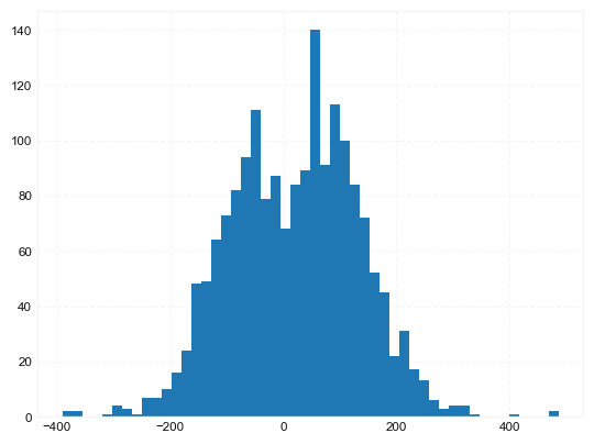
df['CCI20'].hist(bins=50)
<AxesSubplot:>
#https://github.com/matplotlib/mplfinance
#this package help visualize financial data
import mplfinance as mpf
import matplotlib.colors as mcolors

# all_colors = list(mcolors.CSS4_COLORS.keys())#"CSS Colors"
all_colors = list(mcolors.TABLEAU_COLORS.keys()) # "Tableau Palette",
# all_colors = list(mcolors.BASE_COLORS.keys()) #"Base Colors",


#https://github.com/matplotlib/mplfinance/issues/181#issuecomment-667252575
#list of colors: https://matplotlib.org/stable/gallery/color/named_colors.html
#https://github.com/matplotlib/mplfinance/blob/master/examples/styles.ipynb

def make_3panels2(main_data, mid_panel, chart_type='candle', names=None,
                  figratio=(14,9), fill_weights = (0, 0)):
    """
    main chart type: default is candle. alternatives: ohlc, line

    example:
    start = 200

    names = {'main_title': 'MAMA: MESA Adaptive Moving Average',
             'sub_tile': 'S&P 500 (^GSPC)', 'y_tiles': ['price', 'Volume [$10^{6}$]']}


    make_candle(df.iloc[-start:, :5], df.iloc[-start:][['MAMA', 'FAMA']], names = names)

    """

    style = mpf.make_mpf_style(base_mpf_style='yahoo',  #charles
                               base_mpl_style = 'seaborn-whitegrid',
#                                marketcolors=mpf.make_marketcolors(up="r", down="#0000CC",inherit=True),
                               gridcolor="whitesmoke",
                               gridstyle="--", #or None, or - for solid
                               gridaxis="both",
                               edgecolor = 'whitesmoke',
                               facecolor = 'white', #background color within the graph edge
                               figcolor = 'white', #background color outside of the graph edge
                               y_on_right = False,
                               rc =  {'legend.fontsize': 'small',#or number
                                      #'figure.figsize': (14, 9),
                                     'axes.labelsize': 'small',
                                     'axes.titlesize':'small',
                                     'xtick.labelsize':'small',#'x-small', 'small','medium','large'
                                     'ytick.labelsize':'small'
                                     },
                              )

    if (chart_type is None) or (chart_type not in ['ohlc', 'line', 'candle', 'hollow_and_filled']):
        chart_type = 'candle'
    len_dict = {'candle':2, 'ohlc':3, 'line':1, 'hollow_and_filled':2}

    kwargs = dict(type=chart_type, figratio=figratio, volume=True, volume_panel=2,
                  panel_ratios=(4,2,1), tight_layout=True, style=style, returnfig=True)

    if names is None:
        names = {'main_title': '', 'sub_tile': ''}


    added_plots = { }

    fb_bbands2_ = dict(y1=fill_weights[0]*np.ones(mid_panel.shape[0]),
                      y2=fill_weights[1]*np.ones(mid_panel.shape[0]),color="lightskyblue",alpha=0.1,interpolate=True)
    fb_bbands2_['panel'] = 1

    fb_bbands= [fb_bbands2_]


    i = 0
    for name_, data_ in mid_panel.iteritems():
        added_plots[name_] = mpf.make_addplot(data_, panel=1, color=all_colors[i])
        i = i + 1


    fig, axes = mpf.plot(main_data,  **kwargs,
                         addplot=list(added_plots.values()),
                         fill_between=fb_bbands)
    # add a new suptitle
    fig.suptitle(names['main_title'], y=1.05, fontsize=12, x=0.1285)

    axes[0].set_title(names['sub_tile'], fontsize=10, style='italic',  loc='left')
    axes[2].set_ylabel('CCI')

#     axes[0].set_ylabel(names['y_tiles'][0])
#     axes[2].set_ylabel(names['y_tiles'][1])
    return fig, axes
start = -300
end = -200#df.shape[0]
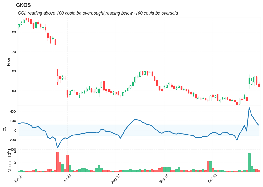
names = {'main_title': f'{ticker}',
'sub_tile': 'CCI: reading above 100 could be overbought;reading below -100 could be oversold'}
aa_, bb_ = make_3panels2(df.iloc[start:end][['Open', 'High', 'Low', 'Close', 'Volume']],
df.iloc[start:end][['CCI20']],
chart_type='hollow_and_filled',names = names,
fill_weights = (-120, 120))