Markov switching dynamic regression models
reference:
- example: https://www.statsmodels.org/dev/examples/notebooks/generated/markov_regression.html
- doc: https://www.statsmodels.org/dev/generated/statsmodels.tsa.regime_switching.markov_regression.MarkovRegression.html
Steps
- download market data using yfinance: download S&P 500 (‘^GSPC')
- calculate return 20 day max return (i.e. target in supervised learning problem):
- for each date (T):
- calculate the max price change in next 20 trading dates: price_change = (max{close price in T+1 to T+20} - {close price on T})/({close price on T})
- create exogenous variables: lagged dependent variable
- lag 1 of target variable
- lag 20 of target varable
Markov switching parameters
- endog: The endogenous variable. the dependent variable (i.e. the target - 20 day max return)
- k_regimes: The number of regimes.
- trend: Whether or not to include a trend. Default is an intercept.
- include an intercept: trend='c'
- include time trend: trend='t'
- include an intercept and time trend: trend='ct'
- no trend: trend='n'
- exog:exogenous regressors
- switching_trend: whether or not all trend coefficients are switching across regimes. Default is True.
- switching_exog:whether or not all regression coefficients are switching across regimes. Default is True.
- switching_variance: Whether or not there is regime-specific heteroskedasticity, i.e. whether or not the error term has a switching variance. Default is False.
Summary
- switching intercept: 2 regimes v. 5 regimes
- set k_regimes as 2 or 5 and leave the rest as default
- switching intercept and lagged dependent variable:
- k_regimes = 3
- lag 1 and lag20 as exog variables
import numpy as np
import pandas as pd
import statsmodels.api as sm

from datetime import datetime, timedelta
import yfinance as yf #to download stock price data
download S&P 500 price data
ticker = '^GSPC'
cur_data = yf.Ticker(ticker)
hist = cur_data.history(period="max")
print(ticker, hist.shape, hist.index.min(), hist.index.max())
^GSPC (19720, 7) 1927-12-30 00:00:00 2021-11-05 00:00:00
df=hist[hist.index>='2000-01-01'].copy(deep=True)
df.head()
| Open | High | Low | Close | Volume | Dividends | Stock Splits |
| Date | | | | | | | |
| 2000-01-03 | 1469.250000 | 1478.000000 | 1438.359985 | 1455.219971 | 931800000 | 0 | 0 |
| 2000-01-04 | 1455.219971 | 1455.219971 | 1397.430054 | 1399.420044 | 1009000000 | 0 | 0 |
| 2000-01-05 | 1399.420044 | 1413.270020 | 1377.680054 | 1402.109985 | 1085500000 | 0 | 0 |
| 2000-01-06 | 1402.109985 | 1411.900024 | 1392.099976 | 1403.449951 | 1092300000 | 0 | 0 |
| 2000-01-07 | 1403.449951 | 1441.469971 | 1400.729980 | 1441.469971 | 1225200000 | 0 | 0 |
calcualte max return in next 20 trading days
#for each stock_id, get the max close in next 20 trading days
price_col = 'Close'
roll_len=20
new_col = 'next_20day_max'
target_list = []

df.sort_index(ascending=True, inplace=True)
df.head(3)
| Open | High | Low | Close | Volume | Dividends | Stock Splits |
| Date | | | | | | | |
| 2000-01-03 | 1469.250000 | 1478.000000 | 1438.359985 | 1455.219971 | 931800000 | 0 | 0 |
| 2000-01-04 | 1455.219971 | 1455.219971 | 1397.430054 | 1399.420044 | 1009000000 | 0 | 0 |
| 2000-01-05 | 1399.420044 | 1413.270020 | 1377.680054 | 1402.109985 | 1085500000 | 0 | 0 |
df_next20dmax=df[[price_col]].shift(1).rolling(roll_len).max()
df_next20dmax.columns=[new_col]
df = df.merge(df_next20dmax, right_index=True, left_index=True, how='inner')

df.dropna(how='any', inplace=True)
df['target']= 100*(df[new_col]-df[price_col])/df[price_col]
| Open | High | Low | Close | Volume | Dividends | Stock Splits | next_20day_max | target |
| Date | | | | | | | | | |
| 2000-02-01 | 1394.459961 | 1412.489990 | 1384.790039 | 1409.280029 | 981000000 | 0 | 0 | 1465.150024 | 3.964435 |
| 2000-02-02 | 1409.280029 | 1420.609985 | 1403.489990 | 1409.119995 | 1038600000 | 0 | 0 | 1465.150024 | 3.976243 |
| 2000-02-03 | 1409.119995 | 1425.780029 | 1398.520020 | 1424.969971 | 1146500000 | 0 | 0 | 1465.150024 | 2.819712 |
df['lag1']=df['target'].shift(1)
df['lag20']=df['target'].shift(20)
df.dropna(how='any', inplace=True)
df.head(3)
| Open | High | Low | Close | Volume | Dividends | Stock Splits | next_20day_max | target | lag1 | lag20 |
| Date | | | | | | | | | | | |
| 2000-03-01 | 1366.420044 | 1383.459961 | 1366.420044 | 1379.189941 | 1274100000 | 0 | 0 | 1441.719971 | 4.533823 | 5.510745 | 3.964435 |
| 2000-03-02 | 1379.189941 | 1386.560059 | 1370.349976 | 1381.760010 | 1198600000 | 0 | 0 | 1441.719971 | 4.339390 | 4.533823 | 3.976243 |
| 2000-03-03 | 1381.760010 | 1410.880005 | 1381.760010 | 1409.170044 | 1150300000 | 0 | 0 | 1441.719971 | 2.309865 | 4.339390 | 2.819712 |
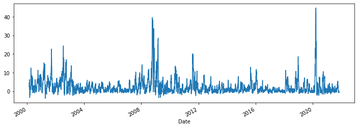
df['target'].plot.line(figsize=(12, 4))
<AxesSubplot:xlabel='Date'>
Markov switching with switching intercept: 2 regimes
- set k_regimes=2: assuming 2 regimes
- leave the rest as default
# Fit the model
# (a switching mean is the default of the MarkovRegession model)
markov_reg = sm.tsa.MarkovRegression(df['target'], k_regimes=2)
res_target = markov_reg.fit()
res_target.summary()
Markov Switching Model Results | Dep. Variable: | target | No. Observations: | 5458 |
| Model: | MarkovRegression | Log Likelihood | -13468.861 |
| Date: | Sat, 06 Nov 2021 | AIC | 26947.723 |
| Time: | 21:37:15 | BIC | 26980.747 |
| Sample: | 0 | HQIC | 26959.246 |
| - 5458 | | |
| Covariance Type: | approx | | |
Regime 0 parameters | coef | std err | z | P>|z| | [0.025 | 0.975] |
| const | 1.6017 | 0.042 | 38.541 | 0.000 | 1.520 | 1.683 |
Regime 1 parameters | coef | std err | z | P>|z| | [0.025 | 0.975] |
| const | 13.3001 | 0.237 | 56.154 | 0.000 | 12.836 | 13.764 |
Non-switching parameters | coef | std err | z | P>|z| | [0.025 | 0.975] |
| sigma2 | 7.5238 | 0.147 | 51.137 | 0.000 | 7.235 | 7.812 |
Regime transition parameters | coef | std err | z | P>|z| | [0.025 | 0.975] |
| p[0->0] | 0.9946 | 0.001 | 923.936 | 0.000 | 0.992 | 0.997 |
| p[1->0] | 0.0701 | 0.014 | 5.182 | 0.000 | 0.044 | 0.097 |
Warnings:
[1] Covariance matrix calculated using numerical (complex-step) differentiation.
-
| note when P> | z | is not small (typically less than 0.05), we accept null hypothesis. |
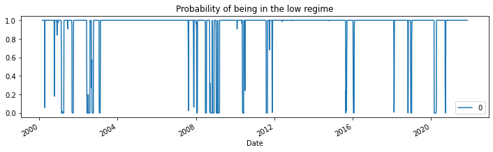
- From the summary output, the first regime (the "low regime") is estimated to be 1.6 whereas in the "high regime" it is 13.3. Below we plot the smoothed probabilities of being in the high regime.
res_target.smoothed_marginal_probabilities[[0]].plot(
    title="Probability of being in the low regime", figsize=(12, 3)
)
res_target.smoothed_marginal_probabilities[[1]].plot(
    title="Probability of being in the high regime", figsize=(12, 3)
)
<AxesSubplot:title={'center':'Probability of being in the high regime'}, xlabel='Date'>
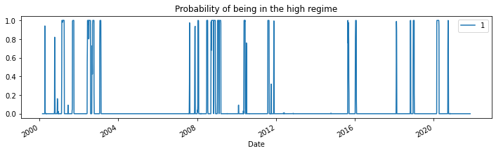
- From the estimated transition matrix we can calculate the expected duration of a low regime versus a high regime.
print(res_target.expected_durations)
[185.00635239 14.26299654]
Markov switching with switching intercept: 5 regimes
- set k_regimes=5: assuming 5 regimes
- leave the rest as default
# Fit the model
# (a switching mean is the default of the MarkovRegession model)
markov_reg = sm.tsa.MarkovRegression(df['target'], k_regimes=5)
res_target = markov_reg.fit()
res_target.summary()
Markov Switching Model Results | Dep. Variable: | target | No. Observations: | 5458 |
| Model: | MarkovRegression | Log Likelihood | -10388.194 |
| Date: | Sat, 06 Nov 2021 | AIC | 20828.388 |
| Time: | 21:39:57 | BIC | 21000.114 |
| Sample: | 0 | HQIC | 20888.309 |
| - 5458 | | |
| Covariance Type: | approx | | |
Regime 0 parameters | coef | std err | z | P>|z| | [0.025 | 0.975] |
| const | 0.5066 | 0.027 | 18.914 | 0.000 | 0.454 | 0.559 |
Regime 1 parameters | coef | std err | z | P>|z| | [0.025 | 0.975] |
| const | 3.5746 | 0.072 | 49.828 | 0.000 | 3.434 | 3.715 |
Regime 2 parameters | coef | std err | z | P>|z| | [0.025 | 0.975] |
| const | 7.7889 | 0.112 | 69.659 | 0.000 | 7.570 | 8.008 |
Regime 3 parameters | coef | std err | z | P>|z| | [0.025 | 0.975] |
| const | 14.8677 | 0.140 | 106.019 | 0.000 | 14.593 | 15.143 |
Regime 4 parameters | coef | std err | z | P>|z| | [0.025 | 0.975] |
| const | 30.9587 | 0.212 | 145.718 | 0.000 | 30.542 | 31.375 |
Non-switching parameters | coef | std err | z | P>|z| | [0.025 | 0.975] |
| sigma2 | 1.7108 | 0.036 | 47.337 | 0.000 | 1.640 | 1.782 |
Regime transition parameters | coef | std err | z | P>|z| | [0.025 | 0.975] |
| p[0->0] | 0.9708 | nan | nan | nan | nan | nan |
| p[1->0] | 0.0780 | 0.001 | 55.775 | 0.000 | 0.075 | 0.081 |
| p[2->0] | 0.0213 | nan | nan | nan | nan | nan |
| p[3->0] | 0.0128 | 0.012 | 1.109 | 0.268 | -0.010 | 0.035 |
| p[4->0] | 8.241e-06 | 0.000 | 0.019 | 0.985 | -0.001 | 0.001 |
| p[0->1] | 0.0278 | 0.001 | 24.099 | 0.000 | 0.026 | 0.030 |
| p[1->1] | 0.8680 | 0.001 | 1313.738 | 0.000 | 0.867 | 0.869 |
| p[2->1] | 0.1157 | 0.005 | 24.987 | 0.000 | 0.107 | 0.125 |
| p[3->1] | 0.0137 | 0.012 | 1.183 | 0.237 | -0.009 | 0.036 |
| p[4->1] | 3.511e-06 | 0.001 | 0.004 | 0.997 | -0.002 | 0.002 |
| p[0->2] | 0.0013 | 0.002 | 0.563 | 0.574 | -0.003 | 0.006 |
| p[1->2] | 0.0540 | nan | nan | nan | nan | nan |
| p[2->2] | 0.8007 | 0.027 | 30.029 | 0.000 | 0.748 | 0.853 |
| p[3->2] | 0.1635 | 6.57e-10 | 2.49e+08 | 0.000 | 0.164 | 0.164 |
| p[4->2] | 1.364e-06 | 0.000 | 0.003 | 0.998 | -0.001 | 0.001 |
| p[0->3] | 1.016e-05 | nan | nan | nan | nan | nan |
| p[1->3] | 6.434e-05 | 0.002 | 0.028 | 0.978 | -0.004 | 0.005 |
| p[2->3] | 0.0623 | 5.27e-07 | 1.18e+05 | 0.000 | 0.062 | 0.062 |
| p[3->3] | 0.8100 | 4.42e-09 | 1.83e+08 | 0.000 | 0.810 | 0.810 |
| p[4->3] | 8.906e-07 | 4.43e-07 | 2.009 | 0.045 | 2.16e-08 | 1.76e-06 |
Warnings:
[1] Covariance matrix calculated using numerical (complex-step) differentiation.
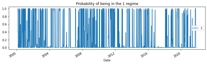
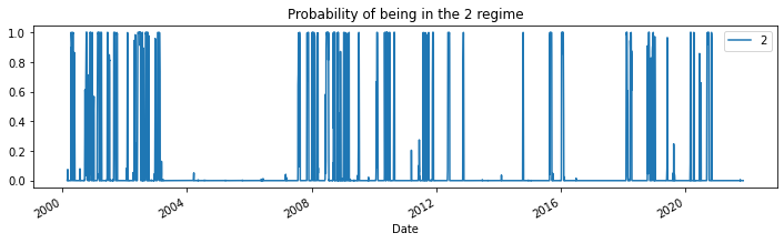
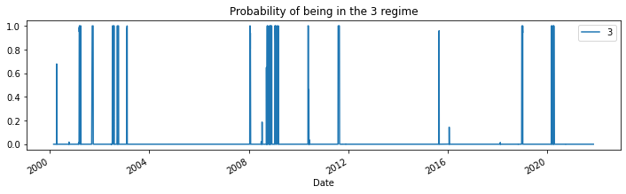
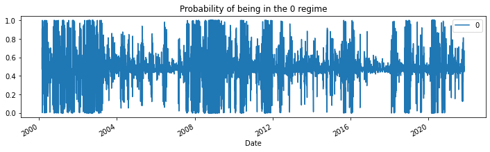
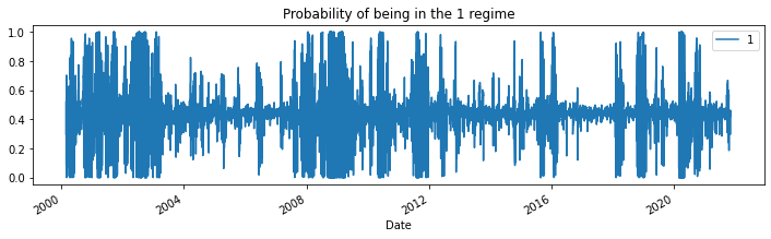
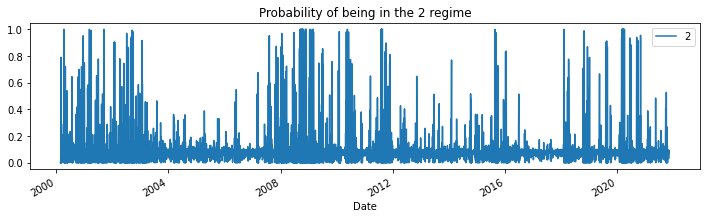
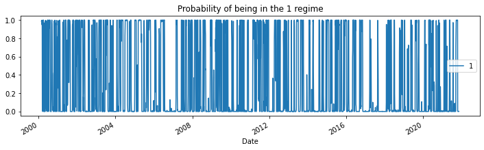
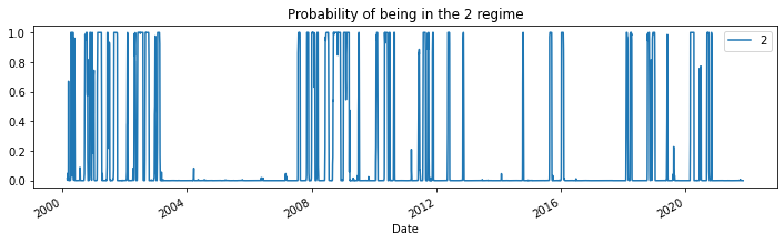
for i in range(5):
    res_target.smoothed_marginal_probabilities[[i]].plot(
        title=f"Probability of being in the {i} regime", figsize=(12, 3)
    )
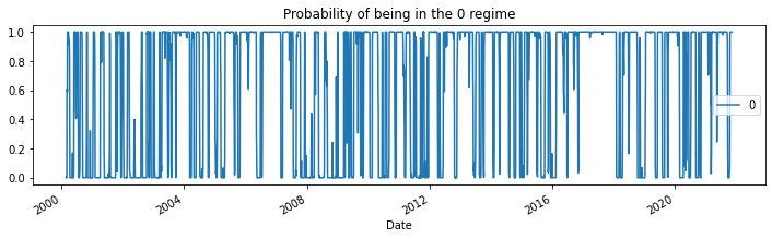
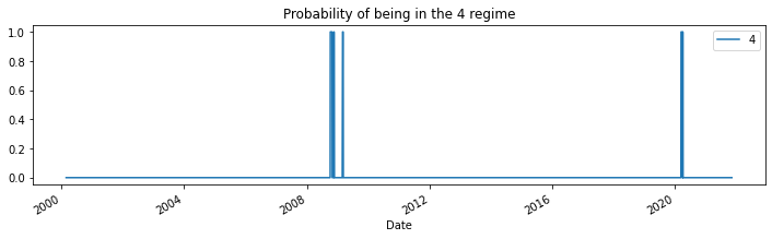
print(res_target.expected_durations)
[3.42706644e+01 7.57564599e+00 5.01865546e+00 5.26380977e+00
 7.13942479e+04]
Markov switching with switching intercept and exogenous variables
- set k_regimes=3: assuming 3 regimes
- lag 1 and lag20 as exogenous variables
- Because the models can be often difficult to estimate, for the 3-regime model we employ a search over starting parameters to improve results, specifying 50 random search repetitions.
# Fit the model
# (a switching mean is the default of the MarkovRegession model)
markov_reg = sm.tsa.MarkovRegression(df['target'], k_regimes=3, exog=df[['lag1', 'lag20']])
res_target = markov_reg.fit()
res_target.summary()
Markov Switching Model Results | Dep. Variable: | target | No. Observations: | 5458 |
| Model: | MarkovRegression | Log Likelihood | -8402.891 |
| Date: | Sat, 06 Nov 2021 | AIC | 16837.782 |
| Time: | 21:40:27 | BIC | 16943.459 |
| Sample: | 0 | HQIC | 16874.656 |
| - 5458 | | |
| Covariance Type: | approx | | |
Regime 0 parameters | coef | std err | z | P>|z| | [0.025 | 0.975] |
| const | 0.2457 | 0.030 | 8.124 | 0.000 | 0.186 | 0.305 |
| x1 | 0.7263 | 0.006 | 121.947 | 0.000 | 0.715 | 0.738 |
| x2 | -0.0624 | 0.006 | -10.622 | 0.000 | -0.074 | -0.051 |
Regime 1 parameters | coef | std err | z | P>|z| | [0.025 | 0.975] |
| const | 0.0278 | 0.034 | 0.821 | 0.412 | -0.039 | 0.094 |
| x1 | 0.9996 | 0.006 | 171.072 | 0.000 | 0.988 | 1.011 |
| x2 | 0.0788 | 0.008 | 9.287 | 0.000 | 0.062 | 0.095 |
Regime 2 parameters | coef | std err | z | P>|z| | [0.025 | 0.975] |
| const | 0.3858 | 0.118 | 3.274 | 0.001 | 0.155 | 0.617 |
| x1 | 1.3538 | 0.014 | 98.518 | 0.000 | 1.327 | 1.381 |
| x2 | 0.0428 | 0.016 | 2.653 | 0.008 | 0.011 | 0.074 |
Non-switching parameters | coef | std err | z | P>|z| | [0.025 | 0.975] |
| sigma2 | 0.8872 | 0.021 | 42.126 | 0.000 | 0.846 | 0.928 |
Regime transition parameters | coef | std err | z | P>|z| | [0.025 | 0.975] |
| p[0->0] | 0.5232 | 0.039 | 13.336 | 0.000 | 0.446 | 0.600 |
| p[1->0] | 0.4120 | 0.029 | 14.022 | 0.000 | 0.354 | 0.470 |
| p[2->0] | 0.3652 | 0.055 | 6.611 | 0.000 | 0.257 | 0.473 |
| p[0->1] | 0.4031 | 0.041 | 9.779 | 0.000 | 0.322 | 0.484 |
| p[1->1] | 0.4723 | 0.034 | 14.089 | 0.000 | 0.407 | 0.538 |
| p[2->1] | 0.5848 | 0.057 | 10.222 | 0.000 | 0.473 | 0.697 |
Warnings:
[1] Covariance matrix calculated using numerical (complex-step) differentiation.
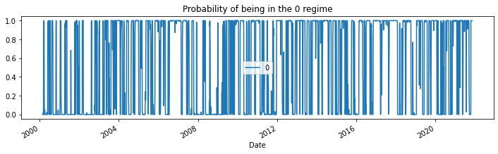
for i in range(3):
    res_target.smoothed_marginal_probabilities[[i]].plot(
        title=f"Probability of being in the {i} regime", figsize=(12, 3)
    )
np.random.seed(5678)

markov_reg = sm.tsa.MarkovRegression(df['target'], k_regimes=3,
                                     trend="c", #{‘n', ‘c', ‘t', ‘ct'}
                                     #switching_trend=False,
                                     #switching_exog=False,
                                     switching_variance=True,
                                     exog=df[['lag20']]
                                    )
res_target = markov_reg.fit(search_reps=50, method='bfgs')
res_target.summary()
Markov Switching Model Results | Dep. Variable: | target | No. Observations: | 5458 |
| Model: | MarkovRegression | Log Likelihood | -9471.406 |
| Date: | Sat, 06 Nov 2021 | AIC | 18972.812 |
| Time: | 21:40:58 | BIC | 19071.885 |
| Sample: | 0 | HQIC | 19007.382 |
| - 5458 | | |
| Covariance Type: | approx | | |
Regime 0 parameters | coef | std err | z | P>|z| | [0.025 | 0.975] |
| const | 0.2896 | 0.018 | 16.545 | 0.000 | 0.255 | 0.324 |
| x1 | -0.0239 | 0.005 | -4.748 | 0.000 | -0.034 | -0.014 |
| sigma2 | 0.4468 | 0.018 | 25.439 | 0.000 | 0.412 | 0.481 |
Regime 1 parameters | coef | std err | z | P>|z| | [0.025 | 0.975] |
| const | 2.9133 | 0.061 | 47.784 | 0.000 | 2.794 | 3.033 |
| x1 | -0.0071 | 0.011 | -0.663 | 0.507 | -0.028 | 0.014 |
| sigma2 | 1.7139 | 0.106 | 16.204 | 0.000 | 1.507 | 1.921 |
Regime 2 parameters | coef | std err | z | P>|z| | [0.025 | 0.975] |
| const | 8.5583 | 0.306 | 27.989 | 0.000 | 7.959 | 9.158 |
| x1 | 0.3187 | 0.043 | 7.347 | 0.000 | 0.234 | 0.404 |
| sigma2 | 36.3329 | 1.987 | 18.285 | 0.000 | 32.438 | 40.227 |
Regime transition parameters | coef | std err | z | P>|z| | [0.025 | 0.975] |
| p[0->0] | 0.9523 | nan | nan | nan | nan | nan |
| p[1->0] | 0.0785 | 0.007 | 11.245 | 0.000 | 0.065 | 0.092 |
| p[2->0] | 0.0029 | 0.003 | 1.114 | 0.265 | -0.002 | 0.008 |
| p[0->1] | 0.0477 | 0.002 | 30.042 | 0.000 | 0.045 | 0.051 |
| p[1->1] | 0.8910 | 0.008 | 106.474 | 0.000 | 0.875 | 0.907 |
| p[2->1] | 0.0673 | 0.010 | 6.811 | 0.000 | 0.048 | 0.087 |
Warnings:
[1] Covariance matrix calculated using numerical (complex-step) differentiation.
for i in range(3):
    res_target.smoothed_marginal_probabilities[[i]].plot(
        title=f"Probability of being in the {i} regime", figsize=(12, 3)
    )
np.random.seed(5678)

markov_reg = sm.tsa.MarkovRegression(df['target'].iloc[:-100], k_regimes=3,
                                     trend="c", #{‘n', ‘c', ‘t', ‘ct'}
                                     #switching_trend=False,
                                     #switching_exog=False,
                                     switching_variance=True,
                                     exog=df[['lag20']].iloc[:-100]
                                    )
res_target = markov_reg.fit(search_reps=50, method='bfgs')
res_target.summary()
Markov Switching Model Results | Dep. Variable: | target | No. Observations: | 5358 |
| Model: | MarkovRegression | Log Likelihood | -9347.917 |
| Date: | Sat, 06 Nov 2021 | AIC | 18725.834 |
| Time: | 21:41:29 | BIC | 18824.629 |
| Sample: | 0 | HQIC | 18760.339 |
| - 5358 | | |
| Covariance Type: | approx | | |
Regime 0 parameters | coef | std err | z | P>|z| | [0.025 | 0.975] |
| const | 0.2965 | 0.018 | 16.736 | 0.000 | 0.262 | 0.331 |
| x1 | -0.0233 | 0.005 | -4.849 | 0.000 | -0.033 | -0.014 |
| sigma2 | 0.4539 | 0.016 | 28.239 | 0.000 | 0.422 | 0.485 |
Regime 1 parameters | coef | std err | z | P>|z| | [0.025 | 0.975] |
| const | 2.9293 | 0.064 | 46.106 | 0.000 | 2.805 | 3.054 |
| x1 | -0.0064 | 0.011 | -0.601 | 0.548 | -0.027 | 0.015 |
| sigma2 | 1.7220 | 0.111 | 15.491 | 0.000 | 1.504 | 1.940 |
Regime 2 parameters | coef | std err | z | P>|z| | [0.025 | 0.975] |
| const | 8.5903 | 0.308 | 27.899 | 0.000 | 7.987 | 9.194 |
| x1 | 0.3182 | 0.043 | 7.435 | 0.000 | 0.234 | 0.402 |
| sigma2 | 36.4287 | 1.965 | 18.542 | 0.000 | 32.578 | 40.279 |
Regime transition parameters | coef | std err | z | P>|z| | [0.025 | 0.975] |
| p[0->0] | 0.9522 | 3.01e-05 | 3.16e+04 | 0.000 | 0.952 | 0.952 |
| p[1->0] | 0.0784 | 0.007 | 11.100 | 0.000 | 0.065 | 0.092 |
| p[2->0] | 0.0029 | 0.003 | 1.146 | 0.252 | -0.002 | 0.008 |
| p[0->1] | 0.0478 | 9.76e-06 | 4895.569 | 0.000 | 0.048 | 0.048 |
| p[1->1] | 0.8905 | 0.009 | 104.534 | 0.000 | 0.874 | 0.907 |
| p[2->1] | 0.0675 | 0.010 | 6.828 | 0.000 | 0.048 | 0.087 |
Warnings:
[1] Covariance matrix calculated using numerical (complex-step) differentiation.