Quick walk through of tsfresh with financial data (Part III)
tsfresh official document page: tsfresh
This notebook uses functions in tsfresh package to create features and select features on financial time series data.
functions in tsfresh package
-
roll_time_seriesfunction: prepare financial time series data to the format of data that can be fed intoextract_featuresfunction. reference extract_featuresfunction: a function that generates hundreds of features from raw time series data. reference- list of features: see here
-
feature_calculatorsmodule: it includes functions such asabs_energyandabsolute_sum_of_changes. All the features that can be generated viaextract_featuresfunction can be individually generated via functions in this module. reference -
imputefunction: impute missing values in generated features. reference select_featuresfunction: select features of high importance to y (i.e. target variable). reference
outline of this notebook
- download data from yahoo finance: download files of two tickers (
PFEandGSK) - load raw csv file: combine two raw csv file into one pandas dataframe, create
idcolumn, and sort the data byDatein ascending order. - prepare data by
roll_time_seriesand create features viaextract_features. imputefunction and deal with missing value- create y (the target variable)
- select features by
select_featuresfunction - save data
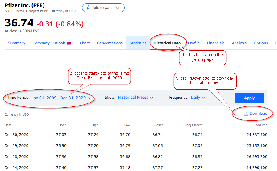
1. download data from yahoo finance
In this notebook, I will use Pfizer Inc. (PFE) and GlaxoSmithKline plc (GSK) as example.
Here shows how to download historical stock price data from yahoo finance. The two downloaded files are named PFE.csv and GSK.csv by default.
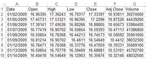
2. load raw csv file
The raw data downloaded from yahoo finance looks like the following screenshot. I will combine PFE.csv and GSK.csv into one pandas dataframe.
import pandas as pd
df1 = pd.read_csv('data/PFE.csv')
df1['id'] = 'PFE'
df1.head(3)
| Date | Open | High | Low | Close | Adj Close | Volume | id | |
|---|---|---|---|---|---|---|---|---|
| 0 | 2009-01-02 | 16.963947 | 17.362429 | 16.793169 | 17.333965 | 10.938112 | 30274000 | PFE |
| 1 | 2009-01-05 | 17.457306 | 17.533207 | 16.963947 | 17.229601 | 10.872255 | 44439200 | PFE |
| 2 | 2009-01-06 | 17.381405 | 17.495256 | 16.802656 | 16.888046 | 10.656727 | 53984400 | PFE |
df2 = pd.read_csv('data/GSK.csv')
df2['id'] = 'GSK'
df2.head(3)
| Date | Open | High | Low | Close | Adj Close | Volume | id | |
|---|---|---|---|---|---|---|---|---|
| 0 | 2009-01-02 | 36.520000 | 37.099998 | 36.439999 | 36.970001 | 19.927216 | 905400 | GSK |
| 1 | 2009-01-05 | 36.110001 | 36.529999 | 35.779999 | 36.380001 | 19.609205 | 1563200 | GSK |
| 2 | 2009-01-06 | 36.880001 | 38.000000 | 36.270000 | 37.759998 | 20.353031 | 2270600 | GSK |
df = pd.concat([df1, df2])
df.head(3)
| Date | Open | High | Low | Close | Adj Close | Volume | id | |
|---|---|---|---|---|---|---|---|---|
| 0 | 2009-01-02 | 16.963947 | 17.362429 | 16.793169 | 17.333965 | 10.938112 | 30274000 | PFE |
| 1 | 2009-01-05 | 17.457306 | 17.533207 | 16.963947 | 17.229601 | 10.872255 | 44439200 | PFE |
| 2 | 2009-01-06 | 17.381405 | 17.495256 | 16.802656 | 16.888046 | 10.656727 | 53984400 | PFE |
df.tail(3)
| Date | Open | High | Low | Close | Adj Close | Volume | id | |
|---|---|---|---|---|---|---|---|---|
| 3017 | 2020-12-28 | 36.790001 | 36.790001 | 36.169998 | 36.290001 | 36.290001 | 2876300 | GSK |
| 3018 | 2020-12-29 | 37.209999 | 37.380001 | 36.860001 | 36.980000 | 36.980000 | 4666300 | GSK |
| 3019 | 2020-12-30 | 37.169998 | 37.240002 | 36.900002 | 37.040001 | 37.040001 | 3071400 | GSK |
print(df1.shape, df2.shape, df.shape)
(3020, 8) (3020, 8) (6040, 8)
del df1
del df2
df.sort_values(by=['id', 'Date'], ascending=[True, True], inplace=True)
df.head(3)
| Date | Open | High | Low | Close | Adj Close | Volume | id | |
|---|---|---|---|---|---|---|---|---|
| 0 | 2009-01-02 | 36.520000 | 37.099998 | 36.439999 | 36.970001 | 19.927216 | 905400 | GSK |
| 1 | 2009-01-05 | 36.110001 | 36.529999 | 35.779999 | 36.380001 | 19.609205 | 1563200 | GSK |
| 2 | 2009-01-06 | 36.880001 | 38.000000 | 36.270000 | 37.759998 | 20.353031 | 2270600 | GSK |
df.tail(3)
| Date | Open | High | Low | Close | Adj Close | Volume | id | |
|---|---|---|---|---|---|---|---|---|
| 3017 | 2020-12-28 | 37.360001 | 37.580002 | 36.680000 | 36.820000 | 36.820000 | 26993700 | PFE |
| 3018 | 2020-12-29 | 36.900002 | 37.200001 | 36.790001 | 37.049999 | 37.049999 | 23152100 | PFE |
| 3019 | 2020-12-30 | 37.029999 | 37.240002 | 36.700001 | 36.740002 | 36.740002 | 24837900 | PFE |
sel_cols = ['id', 'Date', 'Adj Close', 'Volume']
df = df[sel_cols].copy(deep=True)
df.head(3)
| id | Date | Adj Close | Volume | |
|---|---|---|---|---|
| 0 | GSK | 2009-01-02 | 19.927216 | 905400 |
| 1 | GSK | 2009-01-05 | 19.609205 | 1563200 |
| 2 | GSK | 2009-01-06 | 20.353031 | 2270600 |
3. prepare data by `roll_time_series` and create features via `extract_features`
use roll_time_series function to prepare the data: this function convert the data int the following format so it can be consumed by extract_features function.
key parameters of:roll_time_series
- column_id: use
idcolumn - column_sort: use
Datecolumn - max_timeshift: set as 21 (the function will roll 22 rows). This parameter can be set as any integer between 1 to the number of rows in the raw dataframe. I set it as 21 to get features that capture the patterns in the past 30 days (~ 22 business days).
- min_timeshift: set as 21. This parameter must be a number no larger than
max_timeshift. When it is set to less thanmax_timeshift, theroll_time_serieswill roll the data - for the initial few rows of eachid- starting from the row where there aremin_timeshiftof rows to roll. I set this number same asmax_timeshift. - rolling_direction: default value is
1. if set as-1the rolling will be the reverse order.
roll_time_series transforms data in the following format. This function will duplicate rows and increase number of rows to (original_rows_count - 21xnumber of unique id)x22 (i.e. (6040 - 21x2)x22 = 131956)
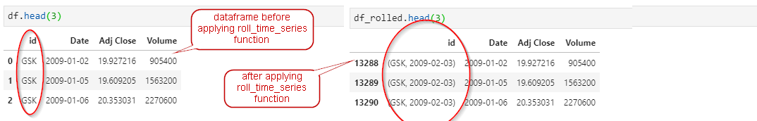
extract_features will turn the dataframe back to original_rows_count - 21 x number of unique id rows.
from tsfresh.utilities.dataframe_functions import roll_time_series
from tsfresh import extract_features
roll_rows = 21
df_rolled = roll_time_series(df, column_id="id", column_sort="Date", max_timeshift=roll_rows, min_timeshift=roll_rows, disable_progressbar=True)
df_features = extract_features(df_rolled, column_id="id", column_sort="Date")
Feature Extraction: 100%|██████████████████████████████████████████████████████████████| 20/20 [03:04<00:00, 9.24s/it]
print(df.shape, df_rolled.shape, df_features.shape, df_features.shape[0]-df.shape[0])
(6040, 4) (131956, 4) (5998, 1558) -42
df_rolled.head(3)
| id | Date | Adj Close | Volume | |
|---|---|---|---|---|
| 0 | (GSK, 2009-02-03) | 2009-01-02 | 19.927216 | 905400 |
| 1 | (GSK, 2009-02-03) | 2009-01-05 | 19.609205 | 1563200 |
| 2 | (GSK, 2009-02-03) | 2009-01-06 | 20.353031 | 2270600 |
df_rolled[df_rolled['Date']=='2009-02-03']
| id | Date | Adj Close | Volume | |
|---|---|---|---|---|
| 21 | (GSK, 2009-02-03) | 2009-02-03 | 19.593031 | 1350600 |
| 64 | (GSK, 2009-02-04) | 2009-02-03 | 19.593031 | 1350600 |
| 107 | (GSK, 2009-02-05) | 2009-02-03 | 19.593031 | 1350600 |
| 150 | (GSK, 2009-02-06) | 2009-02-03 | 19.593031 | 1350600 |
| 193 | (GSK, 2009-02-09) | 2009-02-03 | 19.593031 | 1350600 |
| 236 | (GSK, 2009-02-10) | 2009-02-03 | 19.593031 | 1350600 |
| 279 | (GSK, 2009-02-11) | 2009-02-03 | 19.593031 | 1350600 |
| 322 | (GSK, 2009-02-12) | 2009-02-03 | 19.593031 | 1350600 |
| 365 | (GSK, 2009-02-13) | 2009-02-03 | 19.593031 | 1350600 |
| 408 | (GSK, 2009-02-17) | 2009-02-03 | 19.593031 | 1350600 |
| 451 | (GSK, 2009-02-18) | 2009-02-03 | 19.593031 | 1350600 |
| 494 | (GSK, 2009-02-19) | 2009-02-03 | 19.593031 | 1350600 |
| 537 | (GSK, 2009-02-20) | 2009-02-03 | 19.593031 | 1350600 |
| 580 | (GSK, 2009-02-23) | 2009-02-03 | 19.593031 | 1350600 |
| 623 | (GSK, 2009-02-24) | 2009-02-03 | 19.593031 | 1350600 |
| 666 | (GSK, 2009-02-25) | 2009-02-03 | 19.593031 | 1350600 |
| 709 | (GSK, 2009-02-26) | 2009-02-03 | 19.593031 | 1350600 |
| 752 | (GSK, 2009-02-27) | 2009-02-03 | 19.593031 | 1350600 |
| 795 | (GSK, 2009-03-02) | 2009-02-03 | 19.593031 | 1350600 |
| 838 | (GSK, 2009-03-03) | 2009-02-03 | 19.593031 | 1350600 |
| 881 | (GSK, 2009-03-04) | 2009-02-03 | 19.593031 | 1350600 |
| 924 | (GSK, 2009-03-05) | 2009-02-03 | 19.593031 | 1350600 |
| 43 | (PFE, 2009-02-03) | 2009-02-03 | 9.100128 | 66814700 |
| 86 | (PFE, 2009-02-04) | 2009-02-03 | 9.100128 | 66814700 |
| 129 | (PFE, 2009-02-05) | 2009-02-03 | 9.100128 | 66814700 |
| 172 | (PFE, 2009-02-06) | 2009-02-03 | 9.100128 | 66814700 |
| 215 | (PFE, 2009-02-09) | 2009-02-03 | 9.100128 | 66814700 |
| 258 | (PFE, 2009-02-10) | 2009-02-03 | 9.100128 | 66814700 |
| 301 | (PFE, 2009-02-11) | 2009-02-03 | 9.100128 | 66814700 |
| 344 | (PFE, 2009-02-12) | 2009-02-03 | 9.100128 | 66814700 |
| 387 | (PFE, 2009-02-13) | 2009-02-03 | 9.100128 | 66814700 |
| 430 | (PFE, 2009-02-17) | 2009-02-03 | 9.100128 | 66814700 |
| 473 | (PFE, 2009-02-18) | 2009-02-03 | 9.100128 | 66814700 |
| 516 | (PFE, 2009-02-19) | 2009-02-03 | 9.100128 | 66814700 |
| 559 | (PFE, 2009-02-20) | 2009-02-03 | 9.100128 | 66814700 |
| 602 | (PFE, 2009-02-23) | 2009-02-03 | 9.100128 | 66814700 |
| 645 | (PFE, 2009-02-24) | 2009-02-03 | 9.100128 | 66814700 |
| 688 | (PFE, 2009-02-25) | 2009-02-03 | 9.100128 | 66814700 |
| 731 | (PFE, 2009-02-26) | 2009-02-03 | 9.100128 | 66814700 |
| 774 | (PFE, 2009-02-27) | 2009-02-03 | 9.100128 | 66814700 |
| 817 | (PFE, 2009-03-02) | 2009-02-03 | 9.100128 | 66814700 |
| 860 | (PFE, 2009-03-03) | 2009-02-03 | 9.100128 | 66814700 |
| 903 | (PFE, 2009-03-04) | 2009-02-03 | 9.100128 | 66814700 |
| 946 | (PFE, 2009-03-05) | 2009-02-03 | 9.100128 | 66814700 |
4. `impute` function and deal with missing value
I will first remove features (i.e. columns) with more than 10% of data missing, and then deal with the remaining features.
The impute function replaces all NaNs and infs inplace. Note this function only accepts numeric features and errors will be triggered if the dataframe passed to this function has non-numeric columns.
df_features.head(2)
| Adj Close__variance_larger_than_standard_deviation | Adj Close__has_duplicate_max | Adj Close__has_duplicate_min | Adj Close__has_duplicate | Adj Close__sum_values | Adj Close__abs_energy | Adj Close__mean_abs_change | Adj Close__mean_change | Adj Close__mean_second_derivative_central | Adj Close__median | ... | Volume__fourier_entropy__bins_2 | Volume__fourier_entropy__bins_3 | Volume__fourier_entropy__bins_5 | Volume__fourier_entropy__bins_10 | Volume__fourier_entropy__bins_100 | Volume__permutation_entropy__dimension_3__tau_1 | Volume__permutation_entropy__dimension_4__tau_1 | Volume__permutation_entropy__dimension_5__tau_1 | Volume__permutation_entropy__dimension_6__tau_1 | Volume__permutation_entropy__dimension_7__tau_1 | ||
|---|---|---|---|---|---|---|---|---|---|---|---|---|---|---|---|---|---|---|---|---|---|---|
| GSK | 2009-02-03 | 0.0 | 0.0 | 0.0 | 0.0 | 431.952223 | 8494.084498 | 0.359854 | -0.015914 | 0.024660 | 19.601118 | ... | 0.286836 | 0.286836 | 0.823959 | 1.424130 | 2.369382 | 1.692281 | 2.260234 | 2.707270 | 2.833213 | 2.772589 |
| 2009-02-04 | 0.0 | 0.0 | 0.0 | 0.0 | 431.763572 | 8486.601509 | 0.351641 | 0.006160 | -0.014957 | 19.601118 | ... | 0.286836 | 0.721464 | 0.983088 | 1.539654 | 2.369382 | 1.748067 | 2.378620 | 2.813355 | 2.833213 | 2.772589 |
2 rows × 1558 columns
na_cnt = df_features.isna().sum().sort_values(ascending=False)
na_cnt.head()
Adj Close__fft_coefficient__attr_"abs"__coeff_47    5998
Volume__fft_coefficient__attr_"real"__coeff_17      5998
Volume__fft_coefficient__attr_"real"__coeff_26      5998
Volume__fft_coefficient__attr_"real"__coeff_25      5998
Volume__fft_coefficient__attr_"real"__coeff_24      5998
dtype: int64
ratio = 0.1
print(ratio*df_features.shape[0])
drop_cols = na_cnt[na_cnt>ratio*df_features.shape[0]].index.tolist()
print('before dropping columns: ', df_features.shape)
df_features.drop(columns=drop_cols, inplace=True)
print('after dropping columns: ', df_features.shape)
599.8000000000001
before dropping columns:  (5998, 1558)
after dropping columns:  (5998, 815)
na_cnt = df_features.isna().sum().sort_values(ascending=False)
na_cnt.head()
Volume__sample_entropy                                245
Adj Close__sample_entropy                             180
Volume__max_langevin_fixed_point__m_3__r_30            18
Volume__friedrich_coefficients__coeff_3__m_3__r_30     18
Volume__friedrich_coefficients__coeff_2__m_3__r_30     18
dtype: int64
from tsfresh.utilities.dataframe_functions import impute
impute(df_features)
na_cnt = df_features.isna().sum().sort_values(ascending=False)
na_cnt.head()
Volume__permutation_entropy__dimension_7__tau_1     0
Adj Close__fft_coefficient__attr_"real"__coeff_4    0
Adj Close__fft_coefficient__attr_"imag"__coeff_2    0
Adj Close__fft_coefficient__attr_"imag"__coeff_1    0
Adj Close__fft_coefficient__attr_"imag"__coeff_0    0
dtype: int64
df_features.reset_index(inplace=True)
df_features.head(2)
| level_0 | level_1 | Adj Close__variance_larger_than_standard_deviation | Adj Close__has_duplicate_max | Adj Close__has_duplicate_min | Adj Close__has_duplicate | Adj Close__sum_values | Adj Close__abs_energy | Adj Close__mean_abs_change | Adj Close__mean_change | ... | Volume__fourier_entropy__bins_2 | Volume__fourier_entropy__bins_3 | Volume__fourier_entropy__bins_5 | Volume__fourier_entropy__bins_10 | Volume__fourier_entropy__bins_100 | Volume__permutation_entropy__dimension_3__tau_1 | Volume__permutation_entropy__dimension_4__tau_1 | Volume__permutation_entropy__dimension_5__tau_1 | Volume__permutation_entropy__dimension_6__tau_1 | Volume__permutation_entropy__dimension_7__tau_1 | |
|---|---|---|---|---|---|---|---|---|---|---|---|---|---|---|---|---|---|---|---|---|---|
| 0 | GSK | 2009-02-03 | 0.0 | 0.0 | 0.0 | 0.0 | 431.952223 | 8494.084498 | 0.359854 | -0.015914 | ... | 0.286836 | 0.286836 | 0.823959 | 1.424130 | 2.369382 | 1.692281 | 2.260234 | 2.707270 | 2.833213 | 2.772589 |
| 1 | GSK | 2009-02-04 | 0.0 | 0.0 | 0.0 | 0.0 | 431.763572 | 8486.601509 | 0.351641 | 0.006160 | ... | 0.286836 | 0.721464 | 0.983088 | 1.539654 | 2.369382 | 1.748067 | 2.378620 | 2.813355 | 2.833213 | 2.772589 |
2 rows × 817 columns
df_features.rename(columns={'level_0':'id', 'level_1':'Date'}, inplace=True)
df_features.head(2)
| id | Date | Adj Close__variance_larger_than_standard_deviation | Adj Close__has_duplicate_max | Adj Close__has_duplicate_min | Adj Close__has_duplicate | Adj Close__sum_values | Adj Close__abs_energy | Adj Close__mean_abs_change | Adj Close__mean_change | ... | Volume__fourier_entropy__bins_2 | Volume__fourier_entropy__bins_3 | Volume__fourier_entropy__bins_5 | Volume__fourier_entropy__bins_10 | Volume__fourier_entropy__bins_100 | Volume__permutation_entropy__dimension_3__tau_1 | Volume__permutation_entropy__dimension_4__tau_1 | Volume__permutation_entropy__dimension_5__tau_1 | Volume__permutation_entropy__dimension_6__tau_1 | Volume__permutation_entropy__dimension_7__tau_1 | |
|---|---|---|---|---|---|---|---|---|---|---|---|---|---|---|---|---|---|---|---|---|---|
| 0 | GSK | 2009-02-03 | 0.0 | 0.0 | 0.0 | 0.0 | 431.952223 | 8494.084498 | 0.359854 | -0.015914 | ... | 0.286836 | 0.286836 | 0.823959 | 1.424130 | 2.369382 | 1.692281 | 2.260234 | 2.707270 | 2.833213 | 2.772589 |
| 1 | GSK | 2009-02-04 | 0.0 | 0.0 | 0.0 | 0.0 | 431.763572 | 8486.601509 | 0.351641 | 0.006160 | ... | 0.286836 | 0.721464 | 0.983088 | 1.539654 | 2.369382 | 1.748067 | 2.378620 | 2.813355 | 2.833213 | 2.772589 |
2 rows × 817 columns
5. create y (the target variable)
Target variable: a binary variable to indicate if the maximum of ‘Adj Close' in the next 30 business days is no less than 4% higher than current date's ‘Adj Close'.
Steps to engineer the target variable:
- calculate the maximum
Adj Closein the next 30 rows (data sorted byDatein ascending order).- denote the maximum
Adj Closein the next 30 rows asmax_adj_close_30 - denote the current date's
Adj Closeascurrent_close
- denote the maximum
- calculate the % change of maximum value compared to current date's value.
- denote the % change as
delta_pct delta_pct = (max_adj_close_30 - current_close)/current_close*100
- denote the % change as
- convert the % change to a binary value
- denote the target variable as
target - if
delta_pct >=5, then thetarget=1, elsetarget=0
- denote the target variable as
df.head()
| id | Date | Adj Close | Volume | |
|---|---|---|---|---|
| 0 | GSK | 2009-01-02 | 19.927216 | 905400 |
| 1 | GSK | 2009-01-05 | 19.609205 | 1563200 |
| 2 | GSK | 2009-01-06 | 20.353031 | 2270600 |
| 3 | GSK | 2009-01-07 | 20.778858 | 1621000 |
| 4 | GSK | 2009-01-08 | 21.150766 | 1837100 |
roll_rows = 30
df_rolled2 = roll_time_series(df, column_id="id", column_sort="Date",
                             max_timeshift=roll_rows, min_timeshift=roll_rows,
                              rolling_direction=-1, disable_progressbar=True)
df_rolled2.head()
| id | Date | Adj Close | Volume | |
|---|---|---|---|---|
| 0 | (GSK, 2009-01-02) | 2009-01-02 | 19.927216 | 905400 |
| 1 | (GSK, 2009-01-02) | 2009-01-05 | 19.609205 | 1563200 |
| 2 | (GSK, 2009-01-02) | 2009-01-06 | 20.353031 | 2270600 |
| 3 | (GSK, 2009-01-02) | 2009-01-07 | 20.778858 | 1621000 |
| 4 | (GSK, 2009-01-02) | 2009-01-08 | 21.150766 | 1837100 |
df_features2 = extract_features(df_rolled2, column_id="id", column_sort="Date", column_value = 'Adj Close')
Feature Extraction: 100%|██████████████████████████████████████████████████████████████| 20/20 [01:41<00:00, 5.09s/it]
df_features2.head()
| Adj Close__variance_larger_than_standard_deviation | Adj Close__has_duplicate_max | Adj Close__has_duplicate_min | Adj Close__has_duplicate | Adj Close__sum_values | Adj Close__abs_energy | Adj Close__mean_abs_change | Adj Close__mean_change | Adj Close__mean_second_derivative_central | Adj Close__median | ... | Adj Close__fourier_entropy__bins_2 | Adj Close__fourier_entropy__bins_3 | Adj Close__fourier_entropy__bins_5 | Adj Close__fourier_entropy__bins_10 | Adj Close__fourier_entropy__bins_100 | Adj Close__permutation_entropy__dimension_3__tau_1 | Adj Close__permutation_entropy__dimension_4__tau_1 | Adj Close__permutation_entropy__dimension_5__tau_1 | Adj Close__permutation_entropy__dimension_6__tau_1 | Adj Close__permutation_entropy__dimension_7__tau_1 | ||
|---|---|---|---|---|---|---|---|---|---|---|---|---|---|---|---|---|---|---|---|---|---|---|
| GSK | 2009-01-02 | 0.0 | 0.0 | 0.0 | 1.0 | 607.464175 | 11919.455113 | 0.332559 | -0.055507 | -0.009214 | 19.609205 | ... | 0.376770 | 0.463414 | 0.822265 | 1.037392 | 2.014036 | 1.523876 | 2.224925 | 2.617929 | 2.991501 | 3.163424 |
| 2009-01-05 | 0.0 | 0.0 | 0.0 | 1.0 | 605.941029 | 11861.070968 | 0.326694 | -0.040171 | -0.010375 | 19.593031 | ... | 0.376770 | 0.376770 | 0.831403 | 1.127483 | 2.100679 | 1.523876 | 2.243613 | 2.637309 | 2.991501 | 3.163424 | |
| 2009-01-06 | 0.0 | 0.0 | 0.0 | 0.0 | 604.539174 | 11808.057642 | 0.308457 | -0.071523 | -0.010734 | 19.474447 | ... | 0.376770 | 0.376770 | 0.831403 | 1.276720 | 2.133382 | 1.551250 | 2.262300 | 2.637309 | 2.938182 | 3.107972 | |
| 2009-01-07 | 0.0 | 0.0 | 0.0 | 0.0 | 601.972734 | 11710.174590 | 0.308289 | -0.099742 | -0.013667 | 19.398584 | ... | 0.376770 | 0.463414 | 0.822265 | 1.160186 | 2.393312 | 1.513303 | 2.262300 | 2.585965 | 2.884863 | 3.052521 | |
| 2009-01-08 | 0.0 | 0.0 | 0.0 | 0.0 | 598.630745 | 11582.458051 | 0.307549 | -0.123797 | -0.002870 | 19.305689 | ... | 0.233792 | 0.463414 | 0.702919 | 1.160186 | 2.166085 | 1.452462 | 2.142622 | 2.534620 | 2.831544 | 2.997069 |
5 rows × 779 columns
sel_cols = ['Adj Close__maximum']
df_target = df_features2[sel_cols].copy(deep=True)
df_target.head(10)
| Adj Close__maximum | ||
|---|---|---|
| GSK | 2009-01-02 | 21.150766 |
| 2009-01-05 | 21.150766 | |
| 2009-01-06 | 21.150766 | |
| 2009-01-07 | 21.150766 | |
| 2009-01-08 | 21.150766 | |
| 2009-01-09 | 20.967508 | |
| 2009-01-12 | 20.730349 | |
| 2009-01-13 | 20.185947 | |
| 2009-01-14 | 20.137426 | |
| 2009-01-15 | 20.137426 |
df_target['max_adj_close_30'] = df_target['Adj Close__maximum'].shift(-1)
df_target.head(10)
| Adj Close__maximum | max_adj_close_30 | ||
|---|---|---|---|
| GSK | 2009-01-02 | 21.150766 | 21.150766 |
| 2009-01-05 | 21.150766 | 21.150766 | |
| 2009-01-06 | 21.150766 | 21.150766 | |
| 2009-01-07 | 21.150766 | 21.150766 | |
| 2009-01-08 | 21.150766 | 20.967508 | |
| 2009-01-09 | 20.967508 | 20.730349 | |
| 2009-01-12 | 20.730349 | 20.185947 | |
| 2009-01-13 | 20.185947 | 20.137426 | |
| 2009-01-14 | 20.137426 | 20.137426 | |
| 2009-01-15 | 20.137426 | 20.137426 |
for i in range(0,10):
    print(df.iloc[i,1], df.iloc[i:(30+i),]['Adj Close'].max())
2009-01-02 21.150766
2009-01-05 21.150766
2009-01-06 21.150766
2009-01-07 21.150766
2009-01-08 21.150766
2009-01-09 20.967508
2009-01-12 20.730349
2009-01-13 20.185947
2009-01-14 20.137426
2009-01-15 20.137426
df_target.reset_index(inplace=True)
df_target.rename(columns={'level_0':'id', 'level_1':'Date'}, inplace=True)
df_target.head(2)
| id | Date | Adj Close__maximum | max_adj_close_30 | |
|---|---|---|---|---|
| 0 | GSK | 2009-01-02 | 21.150766 | 21.150766 |
| 1 | GSK | 2009-01-05 | 21.150766 | 21.150766 |
print(df_target.shape, df.shape)
df_target = df_target.merge(df, on=['id', 'Date'], how='inner')
print(df_target.shape, df.shape)
df_target.head(2)
(5980, 4) (6040, 4)
(5980, 6) (6040, 4)
| id | Date | Adj Close__maximum | max_adj_close_30 | Adj Close | Volume | |
|---|---|---|---|---|---|---|
| 0 | GSK | 2009-01-02 | 21.150766 | 21.150766 | 19.927216 | 905400 |
| 1 | GSK | 2009-01-05 | 21.150766 | 21.150766 | 19.609205 | 1563200 |
df_target['delta_pct'] = (df_target['max_adj_close_30'] - df_target['Adj Close'] )/df_target['Adj Close'] *100
df_target.head(2)
| id | Date | Adj Close__maximum | max_adj_close_30 | Adj Close | Volume | delta_pct | |
|---|---|---|---|---|---|---|---|
| 0 | GSK | 2009-01-02 | 21.150766 | 21.150766 | 19.927216 | 905400 | 6.140095 |
| 1 | GSK | 2009-01-05 | 21.150766 | 21.150766 | 19.609205 | 1563200 | 7.861415 |
df_target['target'] = 0
df_target.loc[df_target['delta_pct']>=5, 'target'] = 1
df_target['target'].value_counts()
0    3506
1    2474
Name: target, dtype: int64
df_target.head()
| id | Date | Adj Close__maximum | max_adj_close_30 | Adj Close | Volume | delta_pct | target | |
|---|---|---|---|---|---|---|---|---|
| 0 | GSK | 2009-01-02 | 21.150766 | 21.150766 | 19.927216 | 905400 | 6.140095 | 1 |
| 1 | GSK | 2009-01-05 | 21.150766 | 21.150766 | 19.609205 | 1563200 | 7.861415 | 1 |
| 2 | GSK | 2009-01-06 | 21.150766 | 21.150766 | 20.353031 | 2270600 | 3.919490 | 0 |
| 3 | GSK | 2009-01-07 | 21.150766 | 21.150766 | 20.778858 | 1621000 | 1.789838 | 0 |
| 4 | GSK | 2009-01-08 | 21.150766 | 20.967508 | 21.150766 | 1837100 | -0.866437 | 0 |
6. select features by `select_features` function
select_features(X, y, test_for_binary_target_binary_feature='fisher', test_for_binary_target_real_feature='mann', test_for_real_target_binary_feature='mann', test_for_real_target_real_feature='kendall', fdr_level=0.05, hypotheses_independent=False, n_jobs=1, show_warnings=False, chunksize=None, ml_task='auto', multiclass=False, n_significant=1)
from tsfresh.feature_selection.selection import select_features
df_target.columns
Index(['id', 'Date', 'Adj Close__maximum', 'max_adj_close_30', 'Adj Close',
       'Volume', 'delta_pct', 'target'],
      dtype='object')
sel_cols = ['id', 'Date', 'target', 'max_adj_close_30', 'delta_pct', 'Adj Close','Volume']
#combine features with target variable
print(df_target.shape, df_features.shape)
df_final = df_target[sel_cols].merge(df_features, on = ['id', 'Date'], how='inner')
print(df_final.shape, df_target.shape, df_features.shape)
(5980, 8) (5998, 817)
(5938, 822) (5980, 8) (5998, 817)
df_final.head()
| id | Date | target | max_adj_close_30 | delta_pct | Adj Close | Volume | Adj Close__variance_larger_than_standard_deviation | Adj Close__has_duplicate_max | Adj Close__has_duplicate_min | ... | Volume__fourier_entropy__bins_2 | Volume__fourier_entropy__bins_3 | Volume__fourier_entropy__bins_5 | Volume__fourier_entropy__bins_10 | Volume__fourier_entropy__bins_100 | Volume__permutation_entropy__dimension_3__tau_1 | Volume__permutation_entropy__dimension_4__tau_1 | Volume__permutation_entropy__dimension_5__tau_1 | Volume__permutation_entropy__dimension_6__tau_1 | Volume__permutation_entropy__dimension_7__tau_1 | |
|---|---|---|---|---|---|---|---|---|---|---|---|---|---|---|---|---|---|---|---|---|---|
| 0 | GSK | 2009-02-03 | 0 | 20.137426 | 2.778513 | 19.593031 | 1350600 | 0.0 | 0.0 | 0.0 | ... | 0.286836 | 0.286836 | 0.823959 | 1.424130 | 2.369382 | 1.692281 | 2.260234 | 2.707270 | 2.833213 | 2.772589 |
| 1 | GSK | 2009-02-04 | 0 | 20.137426 | 2.020719 | 19.738565 | 2432700 | 0.0 | 0.0 | 0.0 | ... | 0.286836 | 0.721464 | 0.983088 | 1.539654 | 2.369382 | 1.748067 | 2.378620 | 2.813355 | 2.833213 | 2.772589 |
| 2 | GSK | 2009-02-05 | 0 | 20.008068 | -0.642376 | 20.137426 | 3323300 | 0.0 | 0.0 | 0.0 | ... | 0.450561 | 0.721464 | 1.098612 | 1.539654 | 2.484907 | 1.735434 | 2.406160 | 2.813355 | 2.833213 | 2.772589 |
| 3 | GSK | 2009-02-06 | 0 | 19.937990 | -0.350249 | 20.008068 | 2266700 | 0.0 | 0.0 | 0.0 | ... | 0.450561 | 0.721464 | 1.118743 | 1.632631 | 2.484907 | 1.752424 | 2.479122 | 2.813355 | 2.833213 | 2.772589 |
| 4 | GSK | 2009-02-09 | 0 | 19.609205 | -1.649038 | 19.937990 | 1254900 | 0.0 | 0.0 | 0.0 | ... | 0.286836 | 0.721464 | 0.983088 | 1.473502 | 2.253858 | 1.752424 | 2.506662 | 2.813355 | 2.833213 | 2.772589 |
5 rows × 822 columns
df_final.isna().sum().sort_values(ascending=False).head(5)
max_adj_close_30                                     1
delta_pct                                            1
Volume__permutation_entropy__dimension_7__tau_1      0
Adj Close__fft_coefficient__attr_"real"__coeff_0     0
Adj Close__fft_coefficient__attr_"real"__coeff_10    0
dtype: int64
print(df_final.shape)
df_final.dropna(how='any', inplace=True)
print(df_final.shape)
df_final.isna().sum().sort_values(ascending=False).head(5)
(5938, 822)
(5937, 822)


Volume__permutation_entropy__dimension_7__tau_1                         0
Adj Close__change_quantiles__f_agg_"var"__isabs_True__qh_1.0__ql_0.8    0
Adj Close__fft_coefficient__attr_"real"__coeff_9                        0
Adj Close__fft_coefficient__attr_"real"__coeff_8                        0
Adj Close__fft_coefficient__attr_"real"__coeff_7                        0
dtype: int64
X = df_final.iloc[:, 5:].copy(deep=True)
y = df_final['target']
print(y[:3])
X.head(3)
0    0
1    0
2    0
Name: target, dtype: int64
| Adj Close | Volume | Adj Close__variance_larger_than_standard_deviation | Adj Close__has_duplicate_max | Adj Close__has_duplicate_min | Adj Close__has_duplicate | Adj Close__sum_values | Adj Close__abs_energy | Adj Close__mean_abs_change | Adj Close__mean_change | ... | Volume__fourier_entropy__bins_2 | Volume__fourier_entropy__bins_3 | Volume__fourier_entropy__bins_5 | Volume__fourier_entropy__bins_10 | Volume__fourier_entropy__bins_100 | Volume__permutation_entropy__dimension_3__tau_1 | Volume__permutation_entropy__dimension_4__tau_1 | Volume__permutation_entropy__dimension_5__tau_1 | Volume__permutation_entropy__dimension_6__tau_1 | Volume__permutation_entropy__dimension_7__tau_1 | |
|---|---|---|---|---|---|---|---|---|---|---|---|---|---|---|---|---|---|---|---|---|---|
| 0 | 19.593031 | 1350600 | 0.0 | 0.0 | 0.0 | 0.0 | 431.952223 | 8494.084498 | 0.359854 | -0.015914 | ... | 0.286836 | 0.286836 | 0.823959 | 1.424130 | 2.369382 | 1.692281 | 2.260234 | 2.707270 | 2.833213 | 2.772589 |
| 1 | 19.738565 | 2432700 | 0.0 | 0.0 | 0.0 | 0.0 | 431.763572 | 8486.601509 | 0.351641 | 0.006160 | ... | 0.286836 | 0.721464 | 0.983088 | 1.539654 | 2.369382 | 1.748067 | 2.378620 | 2.813355 | 2.833213 | 2.772589 |
| 2 | 20.137426 | 3323300 | 0.0 | 0.0 | 0.0 | 0.0 | 432.291793 | 8507.596514 | 0.335214 | -0.010267 | ... | 0.450561 | 0.721464 | 1.098612 | 1.539654 | 2.484907 | 1.735434 | 2.406160 | 2.813355 | 2.833213 | 2.772589 |
3 rows × 817 columns
y = df_final['target']
print(X.shape)
for fdr_level in [0.05, 0.01, 0.005, 0.001, 0.0005, 0.0001, 0.00005, 0.00001, 0.000005, 0.000001, 0.0000005, 0.0000001]:
    df_filtered_binary = select_features(X, y, fdr_level=fdr_level, ml_task='classification')
    print(fdr_level, df_filtered_binary.shape)
(5937, 817)
0.05 (5937, 416)
0.01 (5937, 371)
0.005 (5937, 361)
0.001 (5937, 341)
0.0005 (5937, 331)
0.0001 (5937, 313)
5e-05 (5937, 311)
1e-05 (5937, 296)
5e-06 (5937, 292)
1e-06 (5937, 286)
5e-07 (5937, 282)
1e-07 (5937, 277)
y = df_final['delta_pct']

for fdr_level in [0.05, 0.01, 0.005, 0.001, 0.0005, 0.0001, 0.00005, 0.00001, 0.000005, 0.000001, 0.0000005, 0.0000001]:
    df_filtered_reg = select_features(X, y, fdr_level=fdr_level, ml_task='regression')
    print(fdr_level, df_filtered_reg.shape)
0.05 (5937, 399)
0.01 (5937, 372)
0.005 (5937, 361)
0.001 (5937, 339)
0.0005 (5937, 329)
0.0001 (5937, 317)
5e-05 (5937, 311)
1e-05 (5937, 300)
5e-06 (5937, 296)
1e-06 (5937, 284)
5e-07 (5937, 282)
1e-07 (5937, 275)
binary_cols = df_filtered_binary.columns.tolist()
reg_cols = df_filtered_reg.columns.tolist()
both_cols = list(set(binary_cols+reg_cols))
print(len(binary_cols), len(reg_cols), len(both_cols))
277 275 288
'Adj Close' in both_cols, 'Volume'in both_cols
(True, True)
y_cols = ['id', 'Date', 'target', 'delta_pct']
df_final[y_cols + both_cols].head(3)
| id | Date | target | delta_pct | Volume__cwt_coefficients__coeff_11__w_20__widths_(2, 5, 10, 20) | Volume__change_quantiles__f_agg_"mean"__isabs_True__qh_1.0__ql_0.8 | Adj Close__change_quantiles__f_agg_"mean"__isabs_False__qh_0.6__ql_0.2 | Volume__cwt_coefficients__coeff_0__w_10__widths_(2, 5, 10, 20) | Adj Close__sum_values | Adj Close__cwt_coefficients__coeff_13__w_20__widths_(2, 5, 10, 20) | ... | Adj Close__cwt_coefficients__coeff_1__w_20__widths_(2, 5, 10, 20) | Adj Close__cwt_coefficients__coeff_2__w_10__widths_(2, 5, 10, 20) | Adj Close__minimum | Adj Close__cwt_coefficients__coeff_0__w_10__widths_(2, 5, 10, 20) | Volume__fft_coefficient__attr_"abs"__coeff_0 | Volume__cwt_coefficients__coeff_1__w_20__widths_(2, 5, 10, 20) | Adj Close__cwt_coefficients__coeff_1__w_10__widths_(2, 5, 10, 20) | Volume__cwt_coefficients__coeff_5__w_5__widths_(2, 5, 10, 20) | Volume__mean | Adj Close__linear_trend__attr_"slope" | |
|---|---|---|---|---|---|---|---|---|---|---|---|---|---|---|---|---|---|---|---|---|---|
| 0 | GSK | 2009-02-03 | 0 | 2.778513 | 6.827091e+06 | 320000.0 | -0.007189 | 3.020586e+06 | 431.952223 | 66.731853 | ... | 41.004967 | 44.522909 | 18.374868 | 33.597595 | 40175100.0 | 3.762778e+06 | 39.161548 | 3.142434e+06 | 1.826141e+06 | -0.084799 |
| 1 | GSK | 2009-02-04 | 0 | 2.020719 | 6.985642e+06 | 320000.0 | -0.007189 | 3.318212e+06 | 431.763572 | 66.577759 | ... | 40.883390 | 44.542326 | 18.374868 | 33.716539 | 41702400.0 | 4.073276e+06 | 39.240166 | 3.307973e+06 | 1.895564e+06 | -0.079756 |
| 2 | GSK | 2009-02-05 | 0 | -0.642376 | 7.174840e+06 | 320000.0 | -0.007189 | 3.409041e+06 | 432.291793 | 66.449007 | ... | 40.775041 | 44.568357 | 18.374868 | 33.882053 | 43462500.0 | 4.166172e+06 | 39.343889 | 3.367270e+06 | 1.975568e+06 | -0.073900 |
3 rows × 292 columns
file_name = 'PFE_GSK_final.csv'
df_final[y_cols + both_cols].to_csv('data/'+file_name, sep='|', compression='gzip')