Mayo Clinic - STRIP AI - Exploratory data analysis and Image processing with Pillow (PIL)
Jul 26, 2022
1. Understand the train data
1.1. descriptions of the train data
- data file: train.csv
- fields:
- features
- image_id - A unique identifier for this instance having the form {patient_id}_{image_num}. Corresponds to the image {image_id}.tif.
- center_id - Identifies the medical center where the slide was obtained.
- patient_id - Identifies the patient from whom the slide was obtained.
- image_num - Enumerates images of clots obtained from the same patient.
- target
- label - The etiology of the clot, either CE or LAA. This field is the classification target.
- features
1.2. summary of the train data
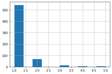
- train data has 754 samples for 632 unique patients:
- the majority have only 1 image
- some patients have as many as 5 images thus 5 samples in the training data
- despite a patient may have more than 1 image, one patient has only one category of etiology (CE or LAA) and only one center_id
- there are total of 11 centers
- most samples are from center 11: 257 out of 754
- center 4 has the 2nd most samples: 114 out of 754
- label
- 72.5% samples are
CEcategory; 27.5% areLAA - 457 patients are
CEcategory, accounts for 72% of all patients. - similar to the overall distribution, the majority are
CEcategory per center_id except center_id = 3 - there are about equal number of samples in
CEandLAAcategories
- 72.5% samples are
1.3. understand the images
-
files sizes:
- most files are less than 500MB; however, there are a few files more than 2GB
- file sizes do not differ much between the 2 categories of clot
CEandLAA - large files are mostly from center 11
-
images:
- explore if images for the same patient can be vastly different
- explore if images for different etiology of the clots look very different
- based on images of two patients, 2 different type of clots look different
2. A bit exploration of the other data
- other.csv - Annotations for images in the other/ folder.
- Has the same fields as train.csv.
- The center_id is unavailable for these images however.
- label - The etiology of the clot, either Unknown or Other.
- other_specified - The specific etiology, when known, in case the etiology is labeled as Other.
3. Image processing with Pillow (PIL)
- the
Pillowpackage (from PIL import Image) offers to resize images in 2 ways: resize and thumbnail- resize images:
- https://pillow.readthedocs.io/en/stable/reference/Image.html?highlight=resize#PIL.Image.Image.resize
- when using resize, you need to calculate the original image height-width ratio and make sure the resized image retains the same ratio.
- Create thumbnails:
- https://pillow.readthedocs.io/en/stable/reference/Image.html?highlight=thumbnail#create-thumbnails
- using thumbnail does not have to deal with the hassle of keeping original image ratio.
- addtional examples and explanations: stackoverflow: How do I resize an image using PIL and maintain its aspect ratio?
- resize images:
- Both thumnail and resize require defining the ‘resample' filter.
- https://pillow.readthedocs.io/en/stable/handbook/concepts.html#concept-filters
- for best quality: choose resampling filter
PIL.Image.LANCZOS - for fastest resizing: choose resampling filter
PIL.Image.NEAREST
- Addtional notes
- Rotate image: when the height of the image is much larger than the width of the image, it may be worthwhile to rotate the image in 90 degrees.
- the rotate method:
transpose(https://pillow.readthedocs.io/en/stable/reference/Image.html?highlight=resize#PIL.Image.Image.resize) - !!! need to assign the transposed image to a new object to make the
transposework. - use
transpose(PIL.Image.Transpose.ROTATE_90)to rotate image in 90 degrees
- the rotate method:
- close image to release memory
- use
close()to destroy the image object and release memory: e.g.img.close() - for the image object, using
del imgandgc.collect()to recycle memory do not help much in releasing the memory
- use
- image attributes
img.sizereturns (width, height) of the image, not (height, width).- to get the height or width, use
img.heightandimg.width
- max pixels to display:
- set
Image.MAX_IMAGE_PIXELS = Noneto disabled the upper limit of pixels to display.
- set
- Rotate image: when the height of the image is much larger than the width of the image, it may be worthwhile to rotate the image in 90 degrees.
Load packages
#basic libs

import pandas as pd
import numpy as np
import os
from pathlib import Path

from datetime import datetime, timedelta
import time
from dateutil.relativedelta import relativedelta

import gc
import copy

#additional data processing

import pyarrow.parquet as pq
import pyarrow as pa

from sklearn.preprocessing import StandardScaler, MinMaxScaler


#visualization
import seaborn as sns
import matplotlib.pyplot as plt

#load images
import matplotlib.image as mpimg
import PIL
from PIL import Image


#settings
pd.options.display.max_rows = 100
pd.options.display.max_columns = 100

Image.MAX_IMAGE_PIXELS = None

import warnings
warnings.filterwarnings("ignore")

import pytorch_lightning as pl
random_seed=1234
pl.seed_everything(random_seed)
1234
import os

next(os.walk('/kaggle/input/mayo-clinic-strip-ai'))
('/kaggle/input/mayo-clinic-strip-ai',
 ['other', 'test', 'train'],
 ['sample_submission.csv', 'train.csv', 'test.csv', 'other.csv'])
Understanding the train data
train_df = pd.read_csv('/kaggle/input/mayo-clinic-strip-ai/train.csv')

print(train_df.shape)
train_df.head(2)
(754, 5)
| image_id | center_id | patient_id | image_num | label | |
|---|---|---|---|---|---|
| 0 | 006388_0 | 11 | 006388 | 0 | CE |
| 1 | 008e5c_0 | 11 | 008e5c | 0 | CE |
patient_id
- most patients have only one image;
- some have as many as 5 iamges.
# check unique number of patients
print(train_df.shape, train_df['patient_id'].nunique())
(754, 5) 632
train_df['patient_id'].value_counts().hist(bins=10)
<AxesSubplot:>
image_num:
- range from 0 to 4, indicating the 1st to the 5th image for a patient
- nearly 84% of samples have image_num=0; less than 5% samples have image_num>=2
a = train_df['image_num'].value_counts().sort_index()

t = pd.concat([a, 100*a/train_df.shape[0]], axis=1)
t.columns = ['# samples', '% of samples']
t.index.name = 'image_num'
display(t)
del a, t
gc.collect()
| # samples | % of samples | |
|---|---|---|
| image_num | ||
| 0 | 632 | 83.819629 |
| 1 | 89 | 11.803714 |
| 2 | 21 | 2.785146 |
| 3 | 8 | 1.061008 |
| 4 | 4 | 0.530504 |
245
train_df['image_num'].value_counts().plot(kind='bar')
<AxesSubplot:>
center_id:
- about 1/3 of samples from center 11
#the center id

a = train_df['center_id'].value_counts().sort_index()

t = pd.concat([a, 100*a/train_df.shape[0]], axis=1)
t.columns = ['# samples', '% of samples']
t.index.name = 'center_id'
display(t)
del a, t
gc.collect()
| # samples | % of samples | |
|---|---|---|
| center_id | ||
| 1 | 54 | 7.161804 |
| 2 | 29 | 3.846154 |
| 3 | 49 | 6.498674 |
| 4 | 114 | 15.119363 |
| 5 | 38 | 5.039788 |
| 6 | 38 | 5.039788 |
| 7 | 99 | 13.129973 |
| 8 | 16 | 2.122016 |
| 9 | 16 | 2.122016 |
| 10 | 44 | 5.835544 |
| 11 | 257 | 34.084881 |
23
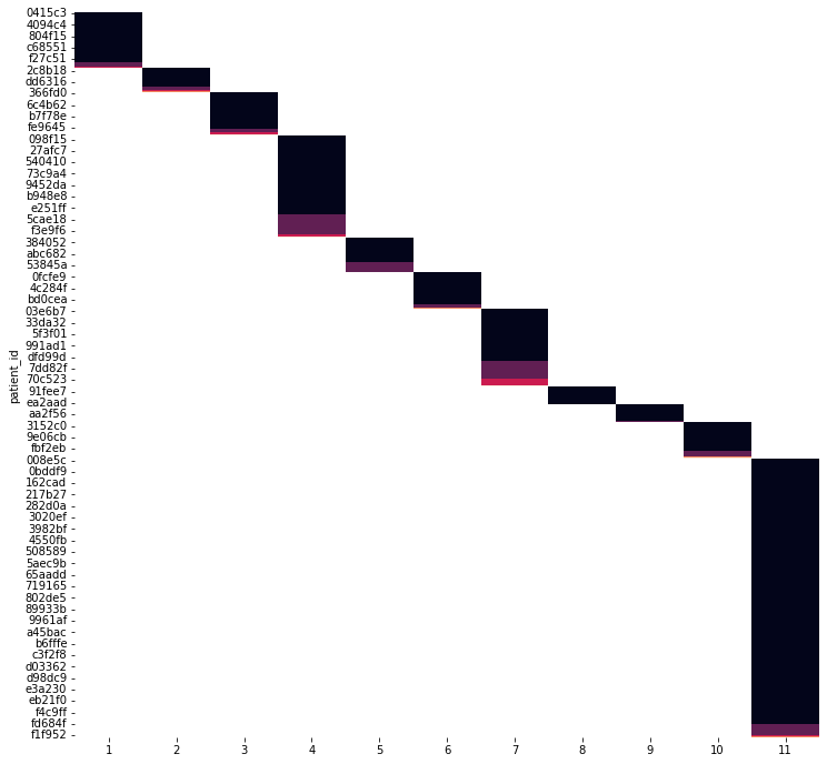
p_center = pd.pivot_table(train_df,
               index='patient_id',
               columns='center_id',
               values=['image_id'],
               aggfunc={'image_id':[np.size]}
              )
p_center.columns = [f'{c}' for _, _, c in p_center.columns]
p_center.isna().sum(axis=1).nunique()
1
p_center.sort_values(by=['1', '2', '3', '4', '5', '6', '7', '8', '9', '10', '11'], inplace=True)

plt.figure(figsize=(12,12))

sns.heatmap(p_center, annot=False, cbar=False)
<AxesSubplot:ylabel='patient_id'>
target varialbe: label
- label
- 72.5% samples are
CEcategory; 27.5% areLAA - 457 patients are
CEcategory, accounts for 72% of all patients.
- 72.5% samples are
- label v center_id
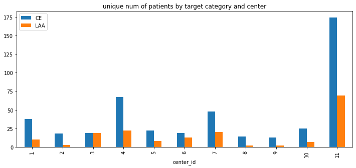
- similar to the overall distribution, the majority are
CEcategory per center_id except center_id = 3 - there are about equal number of samples in
CEandLAAcategories
- similar to the overall distribution, the majority are
#label

a = train_df['label'].value_counts().sort_index()

t = pd.concat([a, 100*a/train_df.shape[0]], axis=1)
t.columns = ['# samples', '% of samples']
t.index.name = 'label'
display(t)
del a, t
gc.collect()
| # samples | % of samples | |
|---|---|---|
| label | ||
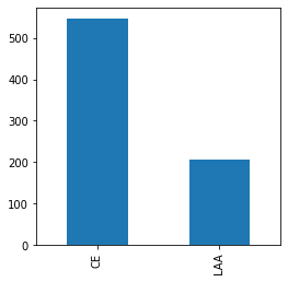
| CE | 547 | 72.546419 |
| LAA | 207 | 27.453581 |
38
train_df['label'].value_counts().plot(kind='bar', figsize=(4,4))
<AxesSubplot:>
#label

a = train_df[['patient_id', 'label']].drop_duplicates(keep='first')['label'].value_counts().sort_index()

t = pd.concat([a, 100*a/train_df['patient_id'].nunique()], axis=1)
t.columns = ['# unique patients', '% of unique patients']
t.index.name = 'label'
display(t)
del a, t
gc.collect()
| # unique patients | % of unique patients | |
|---|---|---|
| label | ||
| CE | 457 | 72.310127 |
| LAA | 175 | 27.689873 |
23
p_label = pd.pivot_table(train_df,
               index='patient_id',
               columns='label',
               values=['image_id'],
               aggfunc={'image_id':[np.size]}
              )
p_label.columns = [f'{c}' for _, _, c in p_label.columns]
# p_label.fillna(value = 0, inplace=True)
p_label['label_cnt'] =2-p_label.isna().sum(axis=1)
p_label['label_cnt'].value_counts()
1    632
Name: label_cnt, dtype: int64
p_label
| CE | LAA | label_cnt | |
|---|---|---|---|
| patient_id | |||
| 006388 | 1.0 | NaN | 1 |
| 008e5c | 1.0 | NaN | 1 |
| 00c058 | NaN | 1.0 | 1 |
| 01adc5 | NaN | 1.0 | 1 |
| 026c97 | 1.0 | NaN | 1 |
| ... | ... | ... | ... |
| fe0cca | 1.0 | NaN | 1 |
| fe9645 | 1.0 | NaN | 1 |
| fe9bec | NaN | 1.0 | 1 |
| ff14e0 | 1.0 | NaN | 1 |
| ffec5c | NaN | 2.0 | 1 |
632 rows × 3 columns
p_label['total']= p_label.sum(axis=1)
p_center = pd.pivot_table(train_df[['center_id', 'label', 'patient_id']].drop_duplicates(keep='first'),
               index='center_id',
               columns='label',
               values=['patient_id'],
               aggfunc={'patient_id':[np.size]}
              )
p_center.columns = [f'{c}' for _, _, c in p_center.columns]
p_center.plot(kind='bar', figsize=(12, 5),
              title='unique num of patients by target category and center')
<AxesSubplot:title={'center':'unique num of patients by target category and center'}, xlabel='center_id'>
Explore the images
-
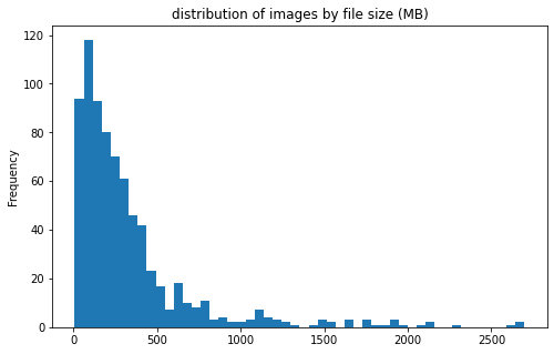
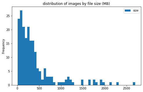
files sizes:
- most files are less than 500MB; however, there are a few files more than 2GB
- file sizes do not differ much between the 2 categories of clot
CEandLAA - large files are mostly from center 11
- image info:
- image width and height distribution
- image ratio (height/width) distribution
- image mode/compression/dpi
- images:
- explore if images for the same patient can be vastly different
- explore if images for different etiology of the clots look very different
- based on images of two patients, 2 different type of clots look different
%%time
#train file sizes

train_pic_folder = '/kaggle/input/mayo-clinic-strip-ai/train'
train_pics = next(os.walk(train_pic_folder))[2]
#
pic_stats = []
for pic in train_pics:
    p = Path(f'{train_pic_folder}/{pic}')
    img = Image.open(f'{train_pic_folder}/{pic}')
    pic_stats.append([pic.split('.')[0], pic, p.stat().st_size/(1024**2), img.width, img.height, img.mode, img.info['compression'], img.info['dpi'] ])
    img.close()
    del img
    gc.collect()

pic_stats_df = pd.DataFrame(data = pic_stats, columns = ['image_id', 'image_name', 'size', 'width', 'height', 'mode', 'compression', 'dpi'])
CPU times: user 4min 8s, sys: 667 ms, total: 4min 8s
Wall time: 4min 9s
pic_stats_df.head(2)
| image_id | image_name | size | width | height | mode | compression | dpi | |
|---|---|---|---|---|---|---|---|---|
| 0 | a4c7df_0 | a4c7df_0.tif | 428.342426 | 30732 | 55283 | RGB | tiff_adobe_deflate | (25.4, 25.4) |
| 1 | f9fc6b_0 | f9fc6b_0.tif | 284.580299 | 38398 | 65388 | RGB | tiff_adobe_deflate | (25.4, 25.4) |
pic_stats_df.sort_values(by='size', ascending=False)
| image_id | image_name | size | width | height | mode | compression | dpi | |
|---|---|---|---|---|---|---|---|---|
| 88 | 6fce60_0 | 6fce60_0.tif | 2697.881285 | 77765 | 39386 | RGB | tiff_adobe_deflate | (50497.015703125, 50497.015703125) |
| 183 | b07b42_0 | b07b42_0.tif | 2665.971151 | 83747 | 47916 | RGB | tiff_adobe_deflate | (50497.015703125, 50497.015703125) |
| 173 | b894f4_0 | b894f4_0.tif | 2641.991510 | 91723 | 45045 | RGB | tiff_adobe_deflate | (50497.015703125, 50497.015703125) |
| 410 | f05449_0 | f05449_0.tif | 2302.191586 | 69789 | 33982 | RGB | tiff_adobe_deflate | (50497.015703125, 50497.015703125) |
| 332 | 288156_0 | 288156_0.tif | 2130.034624 | 97705 | 31890 | RGB | tiff_adobe_deflate | (50497.015703125, 50497.015703125) |
| ... | ... | ... | ... | ... | ... | ... | ... | ... |
| 76 | fd3079_0 | fd3079_0.tif | 11.506842 | 17073 | 22523 | RGB | tiff_adobe_deflate | (25.4, 25.4) |
| 381 | 65fe16_0 | 65fe16_0.tif | 11.114744 | 14695 | 20414 | RGB | tiff_adobe_deflate | (25.4, 25.4) |
| 522 | 70c523_1 | 70c523_1.tif | 10.166765 | 5181 | 20246 | RGB | tiff_adobe_deflate | (25.4, 25.4) |
| 224 | c31442_0 | c31442_0.tif | 9.499516 | 11212 | 31634 | RGB | tiff_adobe_deflate | (25.4, 25.4) |
| 151 | 4ded24_0 | 4ded24_0.tif | 7.027174 | 7220 | 32815 | RGB | tiff_adobe_deflate | (25.4, 25.4) |
754 rows × 8 columns
pic_stats_df['size'].plot(kind='hist', bins=50, figsize = (8, 5),
                          title='distribution of images by file size (MB)')
<AxesSubplot:title={'center':'distribution of images by file size (MB)'}, ylabel='Frequency'>
pic_stats_df.shape, train_df.shape
((754, 8), (754, 5))
train_df = train_df.merge(pic_stats_df, on='image_id', how='left')
train_df.shape
(754, 12)
train_df.head(2)
| image_id | center_id | patient_id | image_num | label | image_name | size | width | height | mode | compression | dpi | |
|---|---|---|---|---|---|---|---|---|---|---|---|---|
| 0 | 006388_0 | 11 | 006388 | 0 | CE | 006388_0.tif | 1252.114786 | 34007 | 60797 | RGB | tiff_adobe_deflate | (25.4, 25.4) |
| 1 | 008e5c_0 | 11 | 008e5c | 0 | CE | 008e5c_0.tif | 104.495459 | 5946 | 29694 | RGB | tiff_adobe_deflate | (25.4, 25.4) |
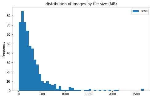
train_df[['label', 'size']].groupby('label').plot(kind='hist', bins=50, figsize = (8, 5),
                          title='distribution of images by file size (MB)')
label
CE     AxesSubplot(0.125,0.125;0.775x0.755)
LAA    AxesSubplot(0.125,0.125;0.775x0.755)
dtype: object
train_df['center_id'] = train_df['center_id'].astype('category')
train_df[['center_id', 'size']].groupby('center_id').plot(kind='hist', bins=50, figsize = (8, 5),
                          title='distribution of images by file size (MB)')
center_id
1     AxesSubplot(0.125,0.125;0.775x0.755)
2     AxesSubplot(0.125,0.125;0.775x0.755)
3     AxesSubplot(0.125,0.125;0.775x0.755)
4     AxesSubplot(0.125,0.125;0.775x0.755)
5     AxesSubplot(0.125,0.125;0.775x0.755)
6     AxesSubplot(0.125,0.125;0.775x0.755)
7     AxesSubplot(0.125,0.125;0.775x0.755)
8     AxesSubplot(0.125,0.125;0.775x0.755)
9     AxesSubplot(0.125,0.125;0.775x0.755)
10    AxesSubplot(0.125,0.125;0.775x0.755)
11    AxesSubplot(0.125,0.125;0.775x0.755)
dtype: object
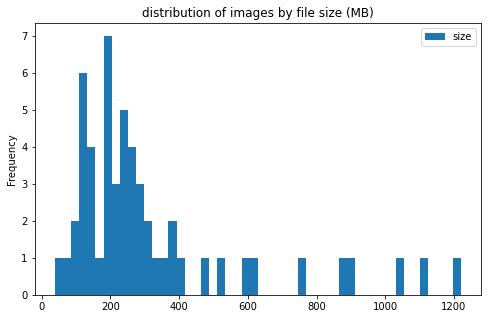
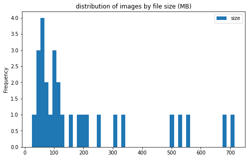
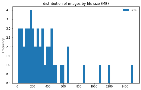
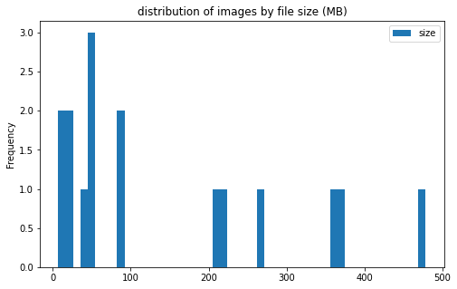
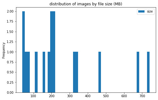
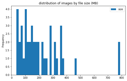
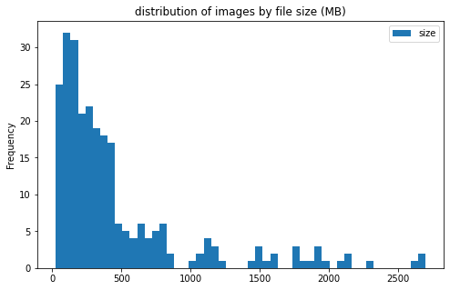
image info
- some images are extremely large (in width and height)
- all images are in
RGBmode and intiff_adobe_deflateformat - only 2 Dots per inches (dpi): (25.4, 25.4) and (50497.015703125, 50497.015703125)
train_df['ratio'] = train_df['height']/train_df['width']
train_df[['height', 'width', 'ratio']].describe()
| height | width | ratio | |
|---|---|---|---|
| count | 754.000000 | 754.000000 | 754.000000 |
| mean | 37622.196286 | 22988.594164 | 2.037926 |
| std | 18058.750676 | 15653.642619 | 1.137743 |
| min | 4470.000000 | 4417.000000 | 0.134461 |
| 25% | 25402.500000 | 13215.250000 | 1.259669 |
| 50% | 34981.500000 | 18700.000000 | 1.924946 |
| 75% | 48919.750000 | 26376.750000 | 2.612830 |
| max | 118076.000000 | 99699.000000 | 8.336422 |
for c in ['height', 'width', 'ratio']:
    train_df[[c]].plot(kind='hist', bins=50)
train_df['mode'].value_counts()
RGB    754
Name: mode, dtype: int64
train_df['compression'].value_counts()
tiff_adobe_deflate    754
Name: compression, dtype: int64
train_df['dpi'].value_counts()
(25.4, 25.4)                          688
(50497.015703125, 50497.015703125)     66
Name: dpi, dtype: int64
images
- explore if images for the same patient can be vastly different
- explore if images for different etiology of the clots look very different
- based on images of two patients, 2 different type of clots look different
#find a patient with at 5 small images
train_df[(train_df['size']<500) & (train_df['image_num']==4)]
| image_id | center_id | patient_id | image_num | label | image_name | size | width | height | mode | compression | dpi | ratio | |
|---|---|---|---|---|---|---|---|---|---|---|---|---|---|
| 29 | 09644e_4 | 10 | 09644e | 4 | CE | 09644e_4.tif | 104.865501 | 9913 | 27715 | RGB | tiff_adobe_deflate | (25.4, 25.4) | 2.795824 |
| 188 | 3d10be_4 | 4 | 3d10be | 4 | CE | 3d10be_4.tif | 33.698559 | 7645 | 9954 | RGB | tiff_adobe_deflate | (25.4, 25.4) | 1.302027 |
| 272 | 56d177_4 | 7 | 56d177 | 4 | CE | 56d177_4.tif | 31.267582 | 15375 | 28006 | RGB | tiff_adobe_deflate | (25.4, 25.4) | 1.821528 |
| 437 | 91b9d3_4 | 3 | 91b9d3 | 4 | LAA | 91b9d3_4.tif | 281.747829 | 27573 | 23032 | RGB | tiff_adobe_deflate | (25.4, 25.4) | 0.835310 |
patient_id='3d10be'
label = 'CE'
train_df[train_df['patient_id']==patient_id]
| image_id | center_id | patient_id | image_num | label | image_name | size | width | height | mode | compression | dpi | ratio | |
|---|---|---|---|---|---|---|---|---|---|---|---|---|---|
| 184 | 3d10be_0 | 4 | 3d10be | 0 | CE | 3d10be_0.tif | 63.952255 | 11088 | 12038 | RGB | tiff_adobe_deflate | (25.4, 25.4) | 1.085678 |
| 185 | 3d10be_1 | 4 | 3d10be | 1 | CE | 3d10be_1.tif | 49.803545 | 9961 | 16650 | RGB | tiff_adobe_deflate | (25.4, 25.4) | 1.671519 |
| 186 | 3d10be_2 | 4 | 3d10be | 2 | CE | 3d10be_2.tif | 49.052773 | 17696 | 13857 | RGB | tiff_adobe_deflate | (25.4, 25.4) | 0.783058 |
| 187 | 3d10be_3 | 4 | 3d10be | 3 | CE | 3d10be_3.tif | 84.386835 | 10533 | 16787 | RGB | tiff_adobe_deflate | (25.4, 25.4) | 1.593753 |
| 188 | 3d10be_4 | 4 | 3d10be | 4 | CE | 3d10be_4.tif | 33.698559 | 7645 | 9954 | RGB | tiff_adobe_deflate | (25.4, 25.4) | 1.302027 |
fig, axes = plt.subplots(nrows=1, ncols=5, figsize=(20, 6))

print(f'patient_id = {patient_id}, label={label}')
for i in range(5):
    img_path = f'/kaggle/input/mayo-clinic-strip-ai/train/{patient_id}_{i}.tif'
    img = Image.open(img_path)
    fac = int(max(img.size)/224)
    h, w = img.size

    axes[i].imshow(img.resize((int(h/fac), int(w/fac))))
    axes[i].set_title(f'{patient_id}_{i}')

    img.close()
    del img, fac
    gc.collect()
patient_id = 3d10be, label=CE
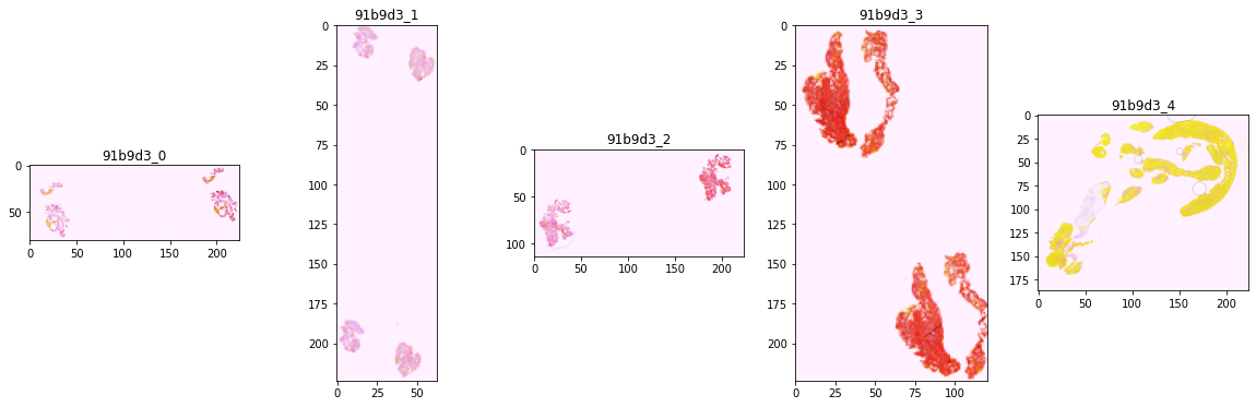
patient_id='91b9d3'
label = 'LAA'
train_df[train_df['patient_id']==patient_id]
| image_id | center_id | patient_id | image_num | label | image_name | size | width | height | mode | compression | dpi | ratio | |
|---|---|---|---|---|---|---|---|---|---|---|---|---|---|
| 433 | 91b9d3_0 | 3 | 91b9d3 | 0 | LAA | 91b9d3_0.tif | 20.182018 | 20047 | 7254 | RGB | tiff_adobe_deflate | (25.4, 25.4) | 0.361850 |
| 434 | 91b9d3_1 | 3 | 91b9d3 | 1 | LAA | 91b9d3_1.tif | 87.481073 | 13081 | 46312 | RGB | tiff_adobe_deflate | (25.4, 25.4) | 3.540402 |
| 435 | 91b9d3_2 | 3 | 91b9d3 | 2 | LAA | 91b9d3_2.tif | 65.516409 | 28704 | 14715 | RGB | tiff_adobe_deflate | (25.4, 25.4) | 0.512646 |
| 436 | 91b9d3_3 | 3 | 91b9d3 | 3 | LAA | 91b9d3_3.tif | 411.783207 | 27426 | 50676 | RGB | tiff_adobe_deflate | (25.4, 25.4) | 1.847736 |
| 437 | 91b9d3_4 | 3 | 91b9d3 | 4 | LAA | 91b9d3_4.tif | 281.747829 | 27573 | 23032 | RGB | tiff_adobe_deflate | (25.4, 25.4) | 0.835310 |
fig, axes = plt.subplots(nrows=1, ncols=5, figsize=(20, 6))

print(f'patient_id = {patient_id}, label={label}')
for i in range(5):
    img_path = f'/kaggle/input/mayo-clinic-strip-ai/train/{patient_id}_{i}.tif'
    img = Image.open(img_path)
    fac = int(max(img.size)/224)
    h, w = img.size

    axes[i].imshow(img.resize((int(h/fac), int(w/fac))))
    axes[i].set_title(f'{patient_id}_{i}')
    img.close()
    del img, fac
    gc.collect()
patient_id = 91b9d3, label=LAA
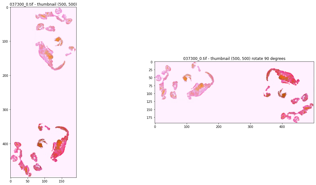
%%time
fig, axes = plt.subplots(nrows=1, ncols=2, figsize=(20, 10))
pic_id = '037300_0.tif'
img = Image.open(f"/kaggle/input/mayo-clinic-strip-ai/train/{pic_id}")
print(img.height, img.width)
img.thumbnail((500, 500), resample=Image.Resampling.LANCZOS, reducing_gap=10)
img2 = img.transpose(PIL.Image.Transpose.ROTATE_90)
axes[0].imshow(img)
axes[0].set_title(f'{pic_id} - thumbnail (500, 500)')
axes[1].imshow(img2)
axes[1].set_title(f'{pic_id} - thumbnail (500, 500) rotate 90 degrees')

img.close()
img2.close()

del img, img2
gc.collect()
70968 27346
CPU times: user 12.6 s, sys: 7.24 s, total: 19.8 s
Wall time: 25.3 s


14548
Others
other_df = pd.read_csv('/kaggle/input/mayo-clinic-strip-ai/other.csv')

print(other_df.shape)
other_df.head(2)
(396, 5)
| image_id | patient_id | image_num | other_specified | label | |
|---|---|---|---|---|---|
| 0 | 01f2b3_0 | 01f2b3 | 0 | NaN | Unknown |
| 1 | 01f2b3_1 | 01f2b3 | 1 | NaN | Unknown |
other_df['label'].value_counts()
Unknown    331
Other       65
Name: label, dtype: int64
#train file sizes

other_pic_folder = '/kaggle/input/mayo-clinic-strip-ai/other'
other_pics = next(os.walk(other_pic_folder))[2]
#
pic_stats = []
for pic in other_pics:
    p = Path(f'{other_pic_folder}/{pic}')
    img = Image.open(f'{other_pic_folder}/{pic}')
    pic_stats.append([pic.split('.')[0], pic, p.stat().st_size/(1024**2), img.width, img.height, img.mode, img.info['compression'], img.info['dpi'] ])

    img.close()
    del img
    gc.collect()

other_pic_stats_df = pd.DataFrame(data = pic_stats, columns = ['image_id', 'image_name', 'size', 'width', 'height', 'mode', 'compression', 'dpi'])
print(other_df.shape, other_pic_stats_df.shape)
other_df = other_df.merge(other_pic_stats_df, on='image_id', how='left')
print(other_df.shape, other_pic_stats_df.shape)
del other_pic_stats_df
gc.collect()
(396, 5) (396, 8)
(396, 12) (396, 8)


23
other_df['other_specified'].value_counts()
Dissection             27
Hypercoagulable        14
PFO                    10
Stent thrombosis        3
Catheter                2
Trauma                  2
Takayasu vasculitis     2
tumor embolization      1
Endocarditis            1
Name: other_specified, dtype: int64
other_df[other_df['other_specified']=='Hypercoagulable']
| image_id | patient_id | image_num | other_specified | label | image_name | size | width | height | mode | compression | dpi | |
|---|---|---|---|---|---|---|---|---|---|---|---|---|
| 4 | 04414e_0 | 04414e | 0 | Hypercoagulable | Other | 04414e_0.tif | 19.079559 | 12656 | 29356 | RGB | tiff_adobe_deflate | (25.4, 25.4) |
| 18 | 0b5827_0 | 0b5827 | 0 | Hypercoagulable | Other | 0b5827_0.tif | 329.594318 | 30721 | 57126 | RGB | tiff_adobe_deflate | (25.4, 25.4) |
| 19 | 0b5827_1 | 0b5827 | 1 | Hypercoagulable | Other | 0b5827_1.tif | 132.289120 | 11005 | 31401 | RGB | tiff_adobe_deflate | (25.4, 25.4) |
| 20 | 0b5827_2 | 0b5827 | 2 | Hypercoagulable | Other | 0b5827_2.tif | 436.645355 | 20804 | 56247 | RGB | tiff_adobe_deflate | (25.4, 25.4) |
| 21 | 0b5827_3 | 0b5827 | 3 | Hypercoagulable | Other | 0b5827_3.tif | 19.248291 | 4841 | 22945 | RGB | tiff_adobe_deflate | (25.4, 25.4) |
| 22 | 0b5827_4 | 0b5827 | 4 | Hypercoagulable | Other | 0b5827_4.tif | 186.556791 | 14304 | 30459 | RGB | tiff_adobe_deflate | (25.4, 25.4) |
| 49 | 222acf_0 | 222acf | 0 | Hypercoagulable | Other | 222acf_0.tif | 203.122671 | 15420 | 27688 | RGB | tiff_adobe_deflate | (25.4, 25.4) |
| 68 | 2e3078_0 | 2e3078 | 0 | Hypercoagulable | Other | 2e3078_0.tif | 154.715866 | 18672 | 36887 | RGB | tiff_adobe_deflate | (25.4, 25.4) |
| 84 | 3aa5ad_0 | 3aa5ad | 0 | Hypercoagulable | Other | 3aa5ad_0.tif | 179.102180 | 19282 | 65462 | RGB | tiff_adobe_deflate | (25.4, 25.4) |
| 96 | 419f30_0 | 419f30 | 0 | Hypercoagulable | Other | 419f30_0.tif | 175.525644 | 15408 | 33227 | RGB | tiff_adobe_deflate | (25.4, 25.4) |
| 123 | 54334d_0 | 54334d | 0 | Hypercoagulable | Other | 54334d_0.tif | 132.995121 | 19792 | 76006 | RGB | tiff_adobe_deflate | (25.4, 25.4) |
| 197 | 8ed18f_0 | 8ed18f | 0 | Hypercoagulable | Other | 8ed18f_0.tif | 59.638159 | 10533 | 49771 | RGB | tiff_adobe_deflate | (25.4, 25.4) |
| 296 | bde458_0 | bde458 | 0 | Hypercoagulable | Other | bde458_0.tif | 60.039425 | 10193 | 31296 | RGB | tiff_adobe_deflate | (25.4, 25.4) |
| 373 | efead4_0 | efead4 | 0 | Hypercoagulable | Other | efead4_0.tif | 53.005348 | 15969 | 29272 | RGB | tiff_adobe_deflate | (25.4, 25.4) |
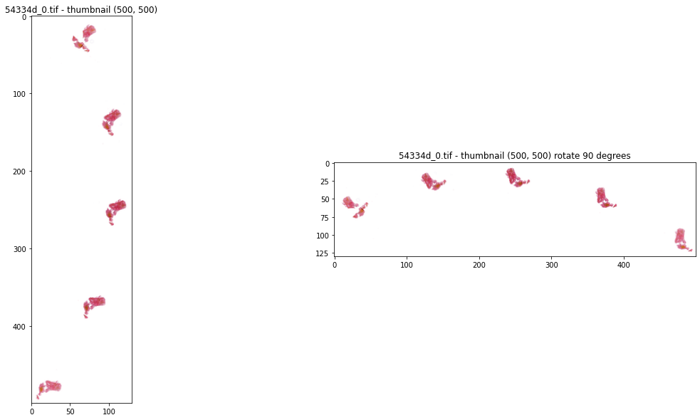
%%time
fig, axes = plt.subplots(nrows=1, ncols=2, figsize=(20, 10))
pic_id = '54334d_0.tif'
img = Image.open(f"/kaggle/input/mayo-clinic-strip-ai/other/{pic_id}")
print(img.height, img.width)
img.thumbnail((500, 500), resample=Image.Resampling.LANCZOS, reducing_gap=10)
img2 = img.transpose(PIL.Image.Transpose.ROTATE_90)
axes[0].imshow(img)
axes[0].set_title(f'{pic_id} - thumbnail (500, 500)')
axes[1].imshow(img2)
axes[1].set_title(f'{pic_id} - thumbnail (500, 500) rotate 90 degrees')

img.close()
img2.close()

del img, img2
gc.collect()
76006 19792
CPU times: user 7.69 s, sys: 5.1 s, total: 12.8 s
Wall time: 14 s


5899