Moving average bands (MAB) and moving average band width (MABW)
References
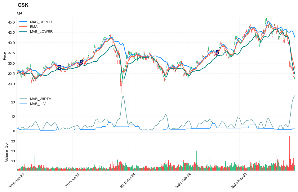
█ OVERVIEW
In "Moving Average Bands" (part 1, July 2021 issue) and "Moving Average Band Width" (part 2, August 2021 issue), author Vitali Apirine explains how moving average bands (MAB) can be used as a trend-following indicator by displaying the movement of a shorter-term moving average in relation to the movement of a longer-term moving average. The distance between the bands will widen as volatility increases and will narrow as volatility decreases.
In part 2, the moving average band width (MABW) measures the percentage difference between the bands. Changes in this difference may indicate a forthcoming move or change in the trend.
█ STRATEGY
- Rules 1:
- Enter when the 10-day moving average (EMA) breaks above the upper MA band
- Exit when the EMA crosses below the lower MA band
- Rules 2:
- Enter when the 10-day moving average (EMA) breaks above the upper MA band, preceded by the moving average band width (MABW) making a 20-day lowest low at least once within the last 10 days
- Exit on a trailing stop of 3 ATRs (14-day) from the trade's highest point
Load basic packages
import pandas as pd
import numpy as np
import os
import gc
import copy
from pathlib import Path
from datetime import datetime, timedelta, time, date
#this package is to download equity price data from yahoo finance
#the source code of this package can be found here: https://github.com/ranaroussi/yfinance/blob/main
import yfinance as yf
pd.options.display.max_rows = 100
pd.options.display.max_columns = 100

import warnings
warnings.filterwarnings("ignore")

import pytorch_lightning as pl
random_seed=1234
pl.seed_everything(random_seed)
Global seed set to 1234


1234
Download data
#S&P 500 (^GSPC),  Dow Jones Industrial Average (^DJI), NASDAQ Composite (^IXIC)
#Russell 2000 (^RUT), Crude Oil Nov 21 (CL=F), Gold Dec 21 (GC=F)
#Treasury Yield 10 Years (^TNX)
#CBOE Volatility Index (^VIX) Chicago Options - Chicago Options Delayed Price. Currency in USD

#benchmark_tickers = ['^GSPC', '^DJI', '^IXIC', '^RUT',  'CL=F', 'GC=F', '^TNX']

benchmark_tickers = ['^GSPC', '^VIX']
tickers = benchmark_tickers + ['GSK', 'BST', 'PFE']
#https://github.com/ranaroussi/yfinance/blob/main/yfinance/base.py
#     def history(self, period="1mo", interval="1d",
#                 start=None, end=None, prepost=False, actions=True,
#                 auto_adjust=True, back_adjust=False,
#                 proxy=None, rounding=False, tz=None, timeout=None, **kwargs):

dfs = {}

for ticker in tickers:
    cur_data = yf.Ticker(ticker)
    hist = cur_data.history(period="max", start='2000-01-01')
    print(datetime.now(), ticker, hist.shape, hist.index.min(), hist.index.max())
    dfs[ticker] = hist
2022-09-10 10:27:39.606085 ^GSPC (5710, 7) 1999-12-31 00:00:00 2022-09-09 00:00:00
2022-09-10 10:27:39.817370 ^VIX (5710, 7) 1999-12-31 00:00:00 2022-09-09 00:00:00
2022-09-10 10:27:40.192326 GSK (5710, 7) 1999-12-31 00:00:00 2022-09-09 00:00:00
2022-09-10 10:27:40.423825 BST (1980, 7) 2014-10-29 00:00:00 2022-09-09 00:00:00
2022-09-10 10:27:40.759307 PFE (5710, 7) 1999-12-31 00:00:00 2022-09-09 00:00:00
ticker = 'GSK'
dfs[ticker].tail(5)
| Open | High | Low | Close | Volume | Dividends | Stock Splits | |
|---|---|---|---|---|---|---|---|
| Date | |||||||
| 2022-09-02 | 31.600000 | 31.969999 | 31.469999 | 31.850000 | 8152600 | 0.0 | 0.0 |
| 2022-09-06 | 31.650000 | 31.760000 | 31.370001 | 31.469999 | 5613900 | 0.0 | 0.0 |
| 2022-09-07 | 31.209999 | 31.590000 | 31.160000 | 31.490000 | 4822000 | 0.0 | 0.0 |
| 2022-09-08 | 30.910000 | 31.540001 | 30.830000 | 31.510000 | 6620900 | 0.0 | 0.0 |
| 2022-09-09 | 31.950001 | 31.969999 | 31.730000 | 31.889999 | 3556800 | 0.0 | 0.0 |
Calculate
from core.finta import TA
df = dfs[ticker][['Open', 'High', 'Low', 'Close', 'Volume']]
df = df.round(2)
TA.MABW
<function core.finta.TA.MABW(ohlc: pandas.core.frame.DataFrame, fast_period: int = 10, slow_period: int = 50, multiplier: float = 1.0, column: str = 'close', adjust: bool = True) -> pandas.core.frame.DataFrame>
df_ta = TA.MABW(df, fast_period = 10, slow_period = 50, multiplier = 1.0)
df = df.merge(df_ta, left_index = True, right_index = True, how='inner' )

del df_ta
gc.collect()
24915
df_ta = TA.EMA(df, period = 20, column="close")
df_ta.name='EMA'
df = df.merge(df_ta, left_index = True, right_index = True, how='inner' )

del df_ta
gc.collect()
21
- Rules 1:
- Enter when the 10-day moving average (EMA) breaks above the upper MA band
- Exit when the EMA crosses below the lower MA band
- Rules 2:
- Enter when the 10-day moving average (EMA) breaks above the upper MA band, preceded by the moving average band width (MABW) making a 20-day lowest low at least once within the last 10 days
- Exit on a trailing stop of 3 ATRs (14-day) from the trade's highest point
df['SIGNAL'] = ((df['EMA']>=df['MAB_UPPER']) & (df['EMA'].shift(1)<df['MAB_UPPER'].shift(1))).astype(int)
df['B'] = df['SIGNAL']*(df["High"] + df["Low"])/2
df['SIGNAL'].value_counts()
0    5675
1      35
Name: SIGNAL, dtype: int64
df['MAB_WIDTH'].rolling(20).min()
Date
1999-12-31         NaN
2000-01-03         NaN
2000-01-04         NaN
2000-01-05         NaN
2000-01-06         NaN
                ...
2022-09-02    3.225288
2022-09-06    3.608219
2022-09-07    4.284088
2022-09-08    5.417958
2022-09-09    6.731750
Name: MAB_WIDTH, Length: 5710, dtype: float64
display(df.head(5))
display(df.tail(5))
| Open | High | Low | Close | Volume | MAB_UPPER | MAB_MIDDLE | MAB_LOWER | MAB_WIDTH | MAB_LLV | EMA | SIGNAL | B | |
|---|---|---|---|---|---|---|---|---|---|---|---|---|---|
| Date | |||||||||||||
| 1999-12-31 | 19.60 | 19.67 | 19.52 | 19.56 | 139400 | NaN | 19.560000 | NaN | NaN | NaN | 19.560000 | 0 | 0.0 |
| 2000-01-03 | 19.58 | 19.71 | 19.25 | 19.45 | 556100 | NaN | 19.499500 | NaN | NaN | NaN | 19.502250 | 0 | 0.0 |
| 2000-01-04 | 19.45 | 19.45 | 18.90 | 18.95 | 367200 | NaN | 19.278605 | NaN | NaN | NaN | 19.299467 | 0 | 0.0 |
| 2000-01-05 | 19.21 | 19.58 | 19.08 | 19.58 | 481700 | NaN | 19.377901 | NaN | NaN | NaN | 19.380453 | 0 | 0.0 |
| 2000-01-06 | 19.38 | 19.43 | 18.90 | 19.30 | 853800 | NaN | 19.355538 | NaN | NaN | NaN | 19.360992 | 0 | 0.0 |
| Open | High | Low | Close | Volume | MAB_UPPER | MAB_MIDDLE | MAB_LOWER | MAB_WIDTH | MAB_LLV | EMA | SIGNAL | B | |
|---|---|---|---|---|---|---|---|---|---|---|---|---|---|
| Date | |||||||||||||
| 2022-09-02 | 31.60 | 31.97 | 31.47 | 31.85 | 8152600 | 41.981303 | 33.059733 | 33.259197 | 23.184605 | 1.291809 | 34.599350 | 0 | 0.0 |
| 2022-09-06 | 31.65 | 31.76 | 31.37 | 31.47 | 5613900 | 41.787135 | 32.770690 | 32.970993 | 23.585774 | 1.291809 | 34.301317 | 0 | 0.0 |
| 2022-09-07 | 31.21 | 31.59 | 31.16 | 31.49 | 4822000 | 41.593738 | 32.537838 | 32.702503 | 23.934548 | 1.291809 | 34.033572 | 0 | 0.0 |
| 2022-09-08 | 30.91 | 31.54 | 30.83 | 31.51 | 6620900 | 41.399202 | 32.350958 | 32.454833 | 24.221746 | 1.291809 | 33.793232 | 0 | 0.0 |
| 2022-09-09 | 31.95 | 31.97 | 31.73 | 31.89 | 3556800 | 41.216672 | 32.267147 | 32.242303 | 24.433689 | 1.291809 | 33.611972 | 0 | 0.0 |
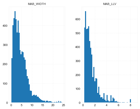
df[['MAB_WIDTH', 'MAB_LLV']].hist(bins=50)
array([[<AxesSubplot:title={'center':'MAB_WIDTH'}>,
        <AxesSubplot:title={'center':'MAB_LLV'}>]], dtype=object)
from core.visuals import *
start = -1000
end = df.shape[0]
df_sub = df.iloc[start:end]
# df_sub = df[(df.index<='2019-04-01') & (df.index>='2019-01-24')]
names = {'main_title': f'{ticker}'}
lines0 = basic_lines(df_sub[['MAB_UPPER', 'EMA', 'MAB_LOWER']],
                     colors = [],
                     **dict(panel=0, width=1.5, secondary_y=False))

lines1 = basic_lines(df_sub[['MAB_WIDTH', 'MAB_LLV']],
                     colors = ['cadetblue'],
                     **dict(panel=1, width=1))

lines2 = basic_lines(df_sub[[ 'B']],
                     colors = ['navy'],
                     **dict(panel=0, type='scatter', marker=r'${B}$' , markersize=100, secondary_y=False))


lines_ = dict(**lines0, **lines1)
lines_.update(lines2)

#shadows_ = basic_shadows(bands=[-0.01, 0.01], nsamples=df.iloc[start:end].shape[0], **dict(panel=1, color="lightskyblue",alpha=0.1,interpolate=True))
shadows_ = []
fig_config_ = dict(figratio=(18,10), volume=True, volume_panel=2,panel_ratios=(4,2, 2), tight_layout=True, returnfig=True,)

ax_cfg_ = {0:dict(basic=[5, 2, ['MAB_UPPER', 'EMA', 'MAB_LOWER']],
                 title=dict(label = 'MA', fontsize=9, style='italic',  loc='left'),
                ),
           2:dict(basic=[2, 0, ['MAB_WIDTH', 'MAB_LLV']]
                ),
          }


names = {'main_title': f'{ticker}'}

aa_, bb_ = make_panels(main_data = df_sub[['Open', 'High', 'Low', 'Close', 'Volume']],
                       added_plots = lines_,
                       fill_betweens = shadows_,
                       fig_config = fig_config_,
                       axes_config = ax_cfg_,
                       names = names)