Detecting High-Volume Breakouts: volume positive negative (VPN)
References
█ OVERVIEW
For this month's Traders' Tips, the focus is Markos Katsanos' article in this issue, "Detecting High-Volume Breakouts." Here, we present the April 2021 Traders' Tips code with possible implementations in various software.
In his article in this issue, "Detecting High-Volume Breakouts," author Markos Katsanos introduces an indicator called volume positive negative (VPN) that attempts to minimize entries in false breakouts. The indicator compares volume on "up" days versus the volume on "down" days and is normalized to oscillate between 100 and -100.
█ STRATEGY
The trading strategy:
setups:
- calculate VPN using period = 30, ema_period = 3
-
calculate RSI using close price and period = 5
- BUY at the next day open when:
- VPN > 10 AND
- RSI < max RSI AND
- close > average of close in period =
- SELL at the next day open when:
- VPN crosses under MA_VPN AND
- Close < Highest( Close, 5 )- 3 * AvgTrueRange( Period )
Strategy:  TASC APR 2021 Strategy
// TASC APR 2021
// Detecting High-Volume Breakouts
// Markos Katsanos

inputs:
    Period( 30 ),
    Smooth( 3 ),
    VPNCrit( 10 ),
    MAB( 30 ),
    RSILen( 5 ),
    MinC( 1 ),
    MinVol( 100000 ),
    MinVolAvgLen( 5 ),
    VolAvgLen( 50 ),
    MinVC( 0.5 ),
    BarToExitOn( 15 ),
    VolDivisor( 1000000 ),
    RSIMaxVal( 90 );

variables:
    VPN( 0 ),
    MAVPN( 0 ),
    RSIVal( 0 ),
    LQD( false ),
    BuyCond1( false );

VPN = XAverage( _TASC_2021_APR_Fx( Period ), Smooth );
MAVPN = Average( VPN, MAB );
RSIVal = RSI( Close, RSILen );

switch ( BarType )
begin
    case 2,3,4: { Daily, Weekly, or Monthly bars }
        // Price, Volume and Liquidity Filter
        LQD = Close > MinC
         and Average( Volume, MinVolAvgLen ) > MinVol
         and Average( Close * Volume, MinVolAvgLen )
          / VolDivisor > MinVC;

        // buy conditions
        BuyCond1 = LQD and
         Average( Volume, VolAvgLen ) >
          Average( Volume, VolAvgLen )[50];

    default: { all other bars }
        // Price, Volume and Liquidity Filter
        LQD = Close > MinC
         and Average( Ticks, MinVolAvgLen ) > MinVol
         and Average( Close * Ticks, MinVolAvgLen )
          / VolDivisor > MinVC;

        // buy conditions
        BuyCond1 = LQD and
         Average( Ticks, VolAvgLen ) >
          Average( Ticks, VolAvgLen )[50];
end;

// buy
if BuyCond1
    and VPN crosses above VPNCrit
    and RSIVal < RSIMaxVal
    and Close > Average( Close, Period ) then
begin
    Buy next bar market;
end;

// sell
if VPN crosses under MAVPN
    and Close < Highest( Close, 5 )
     - 3 * AvgTrueRange( Period ) then
begin
    Sell next bar at market;
end;

// time exit
if BarsSinceEntry = BarToExitOn then
    Sell ( "Time LX" ) next bar at market; ---
Load basic packages
import pandas as pd
import numpy as np
import os
import gc
import copy
from pathlib import Path
from datetime import datetime, timedelta, time, date
#this package is to download equity price data from yahoo finance
#the source code of this package can be found here: https://github.com/ranaroussi/yfinance/blob/main
import yfinance as yf
pd.options.display.max_rows = 100
pd.options.display.max_columns = 100

import warnings
warnings.filterwarnings("ignore")

import pytorch_lightning as pl
random_seed=1234
pl.seed_everything(random_seed)
Global seed set to 1234


1234
Download data
#S&P 500 (^GSPC),  Dow Jones Industrial Average (^DJI), NASDAQ Composite (^IXIC)
#Russell 2000 (^RUT), Crude Oil Nov 21 (CL=F), Gold Dec 21 (GC=F)
#Treasury Yield 10 Years (^TNX)
#CBOE Volatility Index (^VIX) Chicago Options - Chicago Options Delayed Price. Currency in USD

#benchmark_tickers = ['^GSPC', '^DJI', '^IXIC', '^RUT',  'CL=F', 'GC=F', '^TNX']

benchmark_tickers = ['^GSPC', '^VIX']
tickers = benchmark_tickers + ['GSK', 'BST', 'PFE']
#https://github.com/ranaroussi/yfinance/blob/main/yfinance/base.py
#     def history(self, period="1mo", interval="1d",
#                 start=None, end=None, prepost=False, actions=True,
#                 auto_adjust=True, back_adjust=False,
#                 proxy=None, rounding=False, tz=None, timeout=None, **kwargs):

dfs = {}

for ticker in tickers:
    cur_data = yf.Ticker(ticker)
    hist = cur_data.history(period="max", start='2000-01-01')
    print(datetime.now(), ticker, hist.shape, hist.index.min(), hist.index.max())
    dfs[ticker] = hist
2022-09-10 20:13:22.879724 ^GSPC (5710, 7) 1999-12-31 00:00:00 2022-09-09 00:00:00
2022-09-10 20:13:23.187752 ^VIX (5710, 7) 1999-12-31 00:00:00 2022-09-09 00:00:00
2022-09-10 20:13:23.452504 GSK (5710, 7) 1999-12-31 00:00:00 2022-09-09 00:00:00
2022-09-10 20:13:23.567257 BST (1980, 7) 2014-10-29 00:00:00 2022-09-09 00:00:00
2022-09-10 20:13:23.813840 PFE (5710, 7) 1999-12-31 00:00:00 2022-09-09 00:00:00
ticker = 'GSK'
dfs[ticker].tail(5)
| Open | High | Low | Close | Volume | Dividends | Stock Splits | |
|---|---|---|---|---|---|---|---|
| Date | |||||||
| 2022-09-02 | 31.600000 | 31.969999 | 31.469999 | 31.850000 | 8152600 | 0.0 | 0.0 |
| 2022-09-06 | 31.650000 | 31.760000 | 31.370001 | 31.469999 | 5613900 | 0.0 | 0.0 |
| 2022-09-07 | 31.209999 | 31.590000 | 31.160000 | 31.490000 | 4822000 | 0.0 | 0.0 |
| 2022-09-08 | 30.910000 | 31.540001 | 30.830000 | 31.510000 | 6620900 | 0.0 | 0.0 |
| 2022-09-09 | 31.950001 | 31.969999 | 31.730000 | 31.889999 | 3556800 | 0.0 | 0.0 |
Calculate volume positive negative (VPN)
from core.finta import TA
df = dfs[ticker][['Open', 'High', 'Low', 'Close', 'Volume']]
df = df.round(2)
df_ta = TA.VPN(df,  period=30, ema_period=5, mav_period=10)
df = df.merge(df_ta, left_index = True, right_index = True, how='inner' )

del df_ta
gc.collect()
59
df['RSI'] = TA.RSI(df, period = 5, column='close')
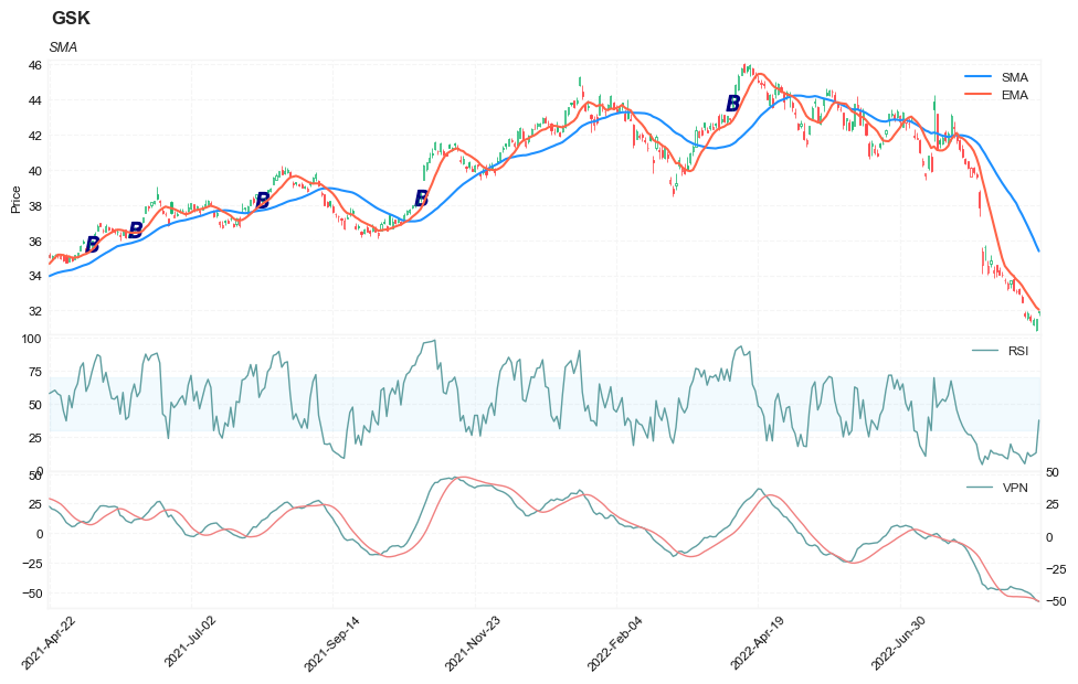
df['SMA'] = TA.SMA(df, period = 30, column='close')
df['EMA'] = TA.SMA(df, period = 9, column='close')
#entry1
# 30-period VPN crosses over 10 AND 5-period RSI < 90 AND close > 30-period SMA
df['SIGNAL'] = ((df['VPN']>10) & (df['VPN'].shift(1)<=10) & (df['RSI']<90) & (df["Close"]>df["SMA"])).astype(int)
df['B'] = df['SIGNAL']*(df["High"] + df["Low"])/2
df['SIGNAL'].value_counts()
0    5636
1      74
Name: SIGNAL, dtype: int64
display(df.head(5))
display(df.tail(5))
| Open | High | Low | Close | Volume | VPN | MA_VPN | RSI | SMA | EMA | SIGNAL | B | |
|---|---|---|---|---|---|---|---|---|---|---|---|---|
| Date | ||||||||||||
| 1999-12-31 | 19.60 | 19.67 | 19.52 | 19.56 | 139400 | NaN | NaN | NaN | NaN | NaN | 0 | 0.0 |
| 2000-01-03 | 19.58 | 19.71 | 19.25 | 19.45 | 556100 | NaN | NaN | 0.000000 | NaN | NaN | 0 | 0.0 |
| 2000-01-04 | 19.45 | 19.45 | 18.90 | 18.95 | 367200 | NaN | NaN | 0.000000 | NaN | NaN | 0 | 0.0 |
| 2000-01-05 | 19.21 | 19.58 | 19.08 | 19.58 | 481700 | NaN | NaN | 57.251908 | NaN | NaN | 0 | 0.0 |
| 2000-01-06 | 19.38 | 19.43 | 18.90 | 19.30 | 853800 | NaN | NaN | 43.436293 | NaN | NaN | 0 | 0.0 |
| Open | High | Low | Close | Volume | VPN | MA_VPN | RSI | SMA | EMA | SIGNAL | B | |
|---|---|---|---|---|---|---|---|---|---|---|---|---|
| Date | ||||||||||||
| 2022-09-02 | 31.60 | 31.97 | 31.47 | 31.85 | 8152600 | -50.125580 | -47.664866 | 13.537814 | 36.800667 | 32.918889 | 0 | 0.0 |
| 2022-09-06 | 31.65 | 31.76 | 31.37 | 31.47 | 5613900 | -51.498332 | -48.032324 | 10.729787 | 36.460333 | 32.667778 | 0 | 0.0 |
| 2022-09-07 | 31.21 | 31.59 | 31.16 | 31.49 | 4822000 | -53.880278 | -48.631443 | 11.931579 | 36.108667 | 32.441111 | 0 | 0.0 |
| 2022-09-08 | 30.91 | 31.54 | 30.83 | 31.51 | 6620900 | -56.951026 | -49.569456 | 13.389069 | 35.724000 | 32.194444 | 0 | 0.0 |
| 2022-09-09 | 31.95 | 31.97 | 31.73 | 31.89 | 3556800 | -57.834300 | -50.835813 | 37.826446 | 35.372000 | 32.050000 | 0 | 0.0 |
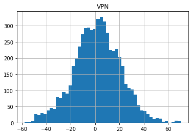
df[['VPN']].hist(bins=50)
array([[<AxesSubplot:title={'center':'VPN'}>]], dtype=object)
from core.visuals import *
start = -350
end = df.shape[0]
df_sub = df.iloc[start:end]
# df_sub = df[(df.index<='2019-04-01') & (df.index>='2019-01-24')]
names = {'main_title': f'{ticker}'}
lines0 = basic_lines(df_sub[['SMA', 'EMA']],
                     colors = [],
                     **dict(panel=0, width=1.5, secondary_y=False))

lines1 = basic_lines(df_sub[['RSI']],
                     colors = ['cadetblue'],
                     **dict(panel=1, width=1))

lines3 = basic_lines(df_sub[['VPN', 'MA_VPN']],
                     colors = ['cadetblue', 'lightcoral'],
                     **dict(panel=2, width=1))

lines2 = basic_lines(df_sub[[ 'B']],
                     colors = ['navy'],
                     **dict(panel=0, type='scatter', marker=r'${B}$' , markersize=100, secondary_y=False))


lines_ = dict(**lines0, **lines1)
lines_.update(lines2)
lines_.update(lines3)

shadows_ = basic_shadows(bands=[30, 70], nsamples=df_sub.shape[0], **dict(panel=1, color="lightskyblue",alpha=0.1,interpolate=True))
#shadows_ = []
fig_config_ = dict(figratio=(18,10), volume=False, volume_panel=2,panel_ratios=(4,2, 2), tight_layout=True, returnfig=True,)

ax_cfg_ = {0:dict(basic=[4, 2, ['SMA', 'EMA']],
                 title=dict(label = 'SMA', fontsize=9, style='italic',  loc='left'),
                ),
           2:dict(basic=[1, 0, ['RSI']]
                ),
           4:dict(basic=[2, 0, ['VPN', 'MA_VPN']]
                ),
          }


names = {'main_title': f'{ticker}'}

aa_, bb_ = make_panels(main_data = df_sub[['Open', 'High', 'Low', 'Close', 'Volume']],
                       added_plots = lines_,
                       fill_betweens = shadows_,
                       fig_config = fig_config_,
                       axes_config = ax_cfg_,
                       names = names)
Simulate
TRADE_CONFIG = dict(INIT_CAPITAL = 10000 ,
                    MIN_TRADE_SIZE = 100 ,
                    MAX_TRADE_SIZE = 1000 ,
                    HOLD_DAYS = 40, #max hold days
                    STOP_LOSS = 0.085, #10% drop
                    KEEP_PROFIT = 0.065,
                    MAX_OPEN = 1, #allow only 1 open position
                    COST = 0.0035,
                   )
Entry 1:
30-period VPN crosses over 10 AND 5-period RSI < 90 AND close > 30-period SMA
df['SIGNAL'].value_counts()
0    5636
1      74
Name: SIGNAL, dtype: int64
trades = []
for i in range(df.shape[0]-5):
    row = df.iloc[i]
    if row['SIGNAL']>0:
        print('enter: ', i)
        row_j = df.iloc[i+1]
        item = dict(signal_date = row.name,
                    enter_date = row_j.name,
                    enter_price = row_j['High']
                   )
        for j in range(i+2, min(i+TRADE_CONFIG['HOLD_DAYS'], df.shape[0])):
            row_j = df.iloc[j]
            price_ = row_j['Low']
            pct_chg = price_/item['enter_price']
            if (pct_chg<= (1 - TRADE_CONFIG['STOP_LOSS'])) | (pct_chg >= (1 + TRADE_CONFIG['KEEP_PROFIT'])):
                break

        item['exit_date'] = row_j.name
        item['exit_price'] = price_
        item['hold_days'] = j - i
        i = j
        print('exit:', i)
        trades.append(item)
enter:  209
exit: 236
enter:  287
exit: 302
enter:  330
exit: 369
enter:  370
exit: 409
enter:  441
exit: 476
enter:  460
exit: 477
enter:  827
exit: 837
enter:  860
exit: 886
enter:  870
exit: 883
enter:  917
exit: 931
enter:  1081
exit: 1120
enter:  1185
exit: 1224
enter:  1226
exit: 1265
enter:  1342
exit: 1381
enter:  1364
exit: 1403
enter:  1425
exit: 1464
enter:  1512
exit: 1551
enter:  1538
exit: 1577
enter:  1551
exit: 1589
enter:  1591
exit: 1630
enter:  1771
exit: 1810
enter:  1933
exit: 1972
enter:  1945
exit: 1982
enter:  2016
exit: 2024
enter:  2088
exit: 2127
enter:  2134
exit: 2141
enter:  2265
exit: 2276
enter:  2336
exit: 2358
enter:  2345
exit: 2359
enter:  2446
exit: 2484
enter:  2504
exit: 2534
enter:  2569
exit: 2601
enter:  2583
exit: 2601
enter:  2648
exit: 2687
enter:  2666
exit: 2695
enter:  2688
exit: 2727
enter:  2971
exit: 3010
enter:  3023
exit: 3062
enter:  3097
exit: 3136
enter:  3100
exit: 3139
enter:  3104
exit: 3143
enter:  3277
exit: 3316
enter:  3285
exit: 3324
enter:  3297
exit: 3336
enter:  3385
exit: 3424
enter:  3421
exit: 3460
enter:  3480
exit: 3519
enter:  3534
exit: 3573
enter:  3555
exit: 3587
enter:  3614
exit: 3653
enter:  3751
exit: 3761
enter:  3790
exit: 3826
enter:  3919
exit: 3935
enter:  3971
exit: 4010
enter:  3986
exit: 4025
enter:  3990
exit: 4029
enter:  4098
exit: 4137
enter:  4161
exit: 4200
enter:  4303
exit: 4335
enter:  4461
exit: 4484
enter:  4528
exit: 4567
enter:  4587
exit: 4626
enter:  4634
exit: 4673
enter:  4637
exit: 4676
enter:  4787
exit: 4826
enter:  4791
exit: 4830
enter:  4923
exit: 4962
enter:  5112
exit: 5151
enter:  5270
exit: 5309
enter:  5375
exit: 5414
enter:  5390
exit: 5429
enter:  5435
exit: 5474
enter:  5491
exit: 5530
enter:  5601
exit: 5640
df_trades = pd.DataFrame(data = trades)
df_trades.shape
(74, 6)
def cal_pnl(trade):
    shares = int(TRADE_CONFIG['INIT_CAPITAL']/trade['enter_price'])
    if shares < TRADE_CONFIG['MIN_TRADE_SIZE']:
        shares = 0
    elif shares > TRADE_CONFIG['MAX_TRADE_SIZE']:
        shares = TRADE_CONFIG['MAX_TRADE_SIZE']
    pnl = shares*(trade['exit_price'] - trade['enter_price']) - shares*trade['enter_price']*TRADE_CONFIG['COST']
    return pnl
df_trades['pnl'] = df_trades.apply(lambda x: cal_pnl(x), axis=1)
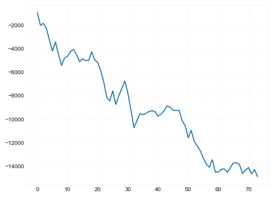
df_trades['pnl'].sum(), (df_trades['pnl']>0).mean()
(-14886.980070000005, 0.44594594594594594)
df_trades
| signal_date | enter_date | enter_price | exit_date | exit_price | hold_days | pnl | |
|---|---|---|---|---|---|---|---|
| 0 | 2000-10-27 | 2000-10-30 | 21.62 | 2000-12-06 | 19.58 | 27 | -977.439540 |
| 1 | 2001-02-21 | 2001-02-22 | 20.67 | 2001-03-14 | 18.56 | 15 | -1054.072635 |
| 2 | 2001-04-24 | 2001-04-25 | 19.46 | 2001-06-19 | 19.83 | 39 | 154.869570 |
| 3 | 2001-06-20 | 2001-06-21 | 20.81 | 2001-08-15 | 19.98 | 39 | -433.360800 |
| 4 | 2001-10-05 | 2001-10-08 | 20.95 | 2001-11-26 | 18.95 | 35 | -988.976025 |
| 5 | 2001-11-01 | 2001-11-02 | 20.51 | 2001-11-27 | 18.70 | 17 | -916.429295 |
| 6 | 2003-04-21 | 2003-04-22 | 15.59 | 2003-05-05 | 16.82 | 10 | 753.453835 |
| 7 | 2003-06-06 | 2003-06-09 | 16.43 | 2003-07-15 | 14.76 | 26 | -1050.323040 |
| 8 | 2003-06-20 | 2003-06-23 | 16.71 | 2003-07-10 | 15.21 | 13 | -931.974030 |
| 9 | 2003-08-27 | 2003-08-28 | 15.54 | 2003-09-17 | 16.57 | 14 | 627.317230 |
| 10 | 2004-04-22 | 2004-04-23 | 17.03 | 2004-06-18 | 17.35 | 39 | 152.851865 |
| 11 | 2004-09-21 | 2004-09-22 | 17.71 | 2004-11-15 | 18.49 | 39 | 404.960460 |
| 12 | 2004-11-17 | 2004-11-18 | 18.45 | 2005-01-13 | 18.82 | 39 | 165.540350 |
| 13 | 2005-05-05 | 2005-05-06 | 21.26 | 2005-06-30 | 20.40 | 39 | -439.172700 |
| 14 | 2005-06-07 | 2005-06-08 | 21.22 | 2005-08-02 | 20.04 | 39 | -590.761170 |
| 15 | 2005-09-01 | 2005-09-02 | 21.13 | 2005-10-27 | 21.72 | 39 | 244.089285 |
| 16 | 2006-01-06 | 2006-01-09 | 22.66 | 2006-03-06 | 22.38 | 39 | -158.455710 |
| 17 | 2006-02-14 | 2006-02-15 | 22.15 | 2006-04-11 | 22.31 | 39 | 37.196225 |
| 18 | 2006-03-06 | 2006-03-07 | 22.63 | 2006-04-28 | 24.32 | 38 | 710.360595 |
| 19 | 2006-05-02 | 2006-05-03 | 24.64 | 2006-06-27 | 23.03 | 39 | -686.977200 |
| 20 | 2007-01-19 | 2007-01-22 | 24.70 | 2007-03-16 | 24.25 | 39 | -216.725800 |
| 21 | 2007-09-11 | 2007-09-12 | 24.67 | 2007-11-05 | 23.07 | 39 | -682.969725 |
| 22 | 2007-09-27 | 2007-09-28 | 24.17 | 2007-11-19 | 21.93 | 37 | -960.057735 |
| 23 | 2008-01-09 | 2008-01-10 | 24.97 | 2008-01-22 | 21.70 | 8 | -1342.958000 |
| 24 | 2008-04-23 | 2008-04-24 | 20.65 | 2008-06-18 | 20.17 | 39 | -267.301100 |
| 25 | 2008-06-27 | 2008-06-30 | 20.92 | 2008-07-09 | 22.77 | 7 | 849.300840 |
| 26 | 2009-01-05 | 2009-01-06 | 18.31 | 2009-01-21 | 16.26 | 11 | -1154.290410 |
| 27 | 2009-04-17 | 2009-04-20 | 14.91 | 2009-05-19 | 16.07 | 22 | 742.236050 |
| 28 | 2009-04-30 | 2009-05-01 | 15.25 | 2009-05-20 | 16.25 | 14 | 620.039375 |
| 29 | 2009-09-23 | 2009-09-24 | 19.78 | 2009-11-16 | 21.10 | 38 | 631.638850 |
| 30 | 2009-12-15 | 2009-12-16 | 21.93 | 2010-01-29 | 19.75 | 30 | -1026.823525 |
| 31 | 2010-03-22 | 2010-03-23 | 20.09 | 2010-05-06 | 17.33 | 32 | -1406.666555 |
| 32 | 2010-04-12 | 2010-04-13 | 20.35 | 2010-05-06 | 17.33 | 18 | -1517.791475 |
| 33 | 2010-07-14 | 2010-07-15 | 19.45 | 2010-09-08 | 20.61 | 39 | 561.249450 |
| 34 | 2010-08-09 | 2010-08-10 | 19.83 | 2010-09-20 | 21.13 | 29 | 620.219880 |
| 35 | 2010-09-09 | 2010-09-10 | 20.86 | 2010-11-03 | 20.75 | 39 | -87.661790 |
| 36 | 2011-10-21 | 2011-10-24 | 24.92 | 2011-12-16 | 25.24 | 39 | 93.344780 |
| 37 | 2012-01-06 | 2012-01-09 | 25.10 | 2012-03-05 | 25.61 | 39 | 168.015700 |
| 38 | 2012-04-24 | 2012-04-25 | 26.40 | 2012-06-19 | 26.68 | 39 | 70.912800 |
| 39 | 2012-04-27 | 2012-04-30 | 26.75 | 2012-06-22 | 26.63 | 39 | -79.682125 |
| 40 | 2012-05-03 | 2012-05-04 | 26.82 | 2012-06-28 | 25.88 | 39 | -384.599640 |
| 41 | 2013-01-11 | 2013-01-14 | 26.37 | 2013-03-11 | 26.88 | 39 | 158.310195 |
| 42 | 2013-01-24 | 2013-01-25 | 26.79 | 2013-03-21 | 27.70 | 39 | 304.455655 |
| 43 | 2013-02-11 | 2013-02-12 | 27.19 | 2013-04-09 | 28.41 | 39 | 412.814445 |
| 44 | 2013-06-18 | 2013-06-19 | 32.07 | 2013-08-13 | 31.75 | 39 | -134.428195 |
| 45 | 2013-08-08 | 2013-08-09 | 31.98 | 2013-10-03 | 31.29 | 39 | -250.202160 |
| 46 | 2013-10-31 | 2013-11-01 | 32.87 | 2013-12-27 | 32.95 | 39 | -10.653680 |
| 47 | 2014-01-21 | 2014-01-22 | 34.37 | 2014-03-18 | 34.56 | 39 | 20.214450 |
| 48 | 2014-02-20 | 2014-02-21 | 35.64 | 2014-04-07 | 32.55 | 32 | -900.127200 |
| 49 | 2014-05-15 | 2014-05-16 | 35.62 | 2014-07-11 | 34.28 | 39 | -410.107600 |
| 50 | 2014-11-28 | 2014-12-01 | 30.99 | 2014-12-12 | 27.91 | 10 | -1026.685730 |
| 51 | 2015-01-27 | 2015-01-28 | 29.99 | 2015-03-19 | 31.95 | 36 | 617.726655 |
| 52 | 2015-07-31 | 2015-08-03 | 29.56 | 2015-08-24 | 26.98 | 16 | -907.009480 |
| 53 | 2015-10-14 | 2015-10-15 | 28.48 | 2015-12-09 | 27.45 | 39 | -396.517680 |
| 54 | 2015-11-04 | 2015-11-05 | 29.16 | 2015-12-31 | 28.05 | 39 | -414.524520 |
| 55 | 2015-11-10 | 2015-11-11 | 28.75 | 2016-01-07 | 27.07 | 39 | -617.876875 |
| 56 | 2016-04-18 | 2016-04-19 | 31.13 | 2016-06-13 | 29.65 | 39 | -510.054555 |
| 57 | 2016-07-18 | 2016-07-19 | 32.00 | 2016-09-12 | 31.23 | 39 | -275.184000 |
| 58 | 2017-02-08 | 2017-02-09 | 29.99 | 2017-03-27 | 32.03 | 32 | 644.366655 |
| 59 | 2017-09-25 | 2017-09-26 | 31.40 | 2017-10-26 | 28.21 | 23 | -1049.368200 |
| 60 | 2017-12-29 | 2018-01-02 | 28.98 | 2018-02-27 | 29.11 | 39 | 9.856650 |
| 61 | 2018-03-27 | 2018-03-28 | 31.74 | 2018-05-22 | 32.56 | 39 | 223.306650 |
| 62 | 2018-06-04 | 2018-06-05 | 32.79 | 2018-07-30 | 33.01 | 39 | 31.991440 |
| 63 | 2018-06-07 | 2018-06-08 | 33.19 | 2018-08-02 | 32.33 | 39 | -293.825665 |
| 64 | 2019-01-11 | 2019-01-14 | 32.09 | 2019-03-11 | 33.51 | 39 | 406.690035 |
| 65 | 2019-01-17 | 2019-01-18 | 32.46 | 2019-03-15 | 33.88 | 39 | 402.368120 |
| 66 | 2019-07-29 | 2019-07-30 | 35.84 | 2019-09-23 | 36.00 | 39 | 9.642240 |
| 67 | 2020-04-28 | 2020-04-29 | 37.46 | 2020-06-23 | 36.98 | 39 | -162.555260 |
| 68 | 2020-12-10 | 2020-12-11 | 34.59 | 2021-02-08 | 32.11 | 39 | -751.707785 |
| 69 | 2021-05-13 | 2021-05-14 | 36.49 | 2021-07-09 | 37.71 | 39 | 299.286090 |
| 70 | 2021-06-04 | 2021-06-07 | 36.76 | 2021-07-30 | 37.65 | 39 | 207.084480 |
| 71 | 2021-08-09 | 2021-08-10 | 38.41 | 2021-10-04 | 36.48 | 39 | -536.753100 |
| 72 | 2021-10-27 | 2021-10-28 | 40.28 | 2021-12-22 | 41.86 | 39 | 356.876960 |
| 73 | 2022-04-05 | 2022-04-06 | 44.86 | 2022-06-01 | 42.33 | 39 | -596.516220 |
df_trades['pnl'].cumsum().plot()
<AxesSubplot:>
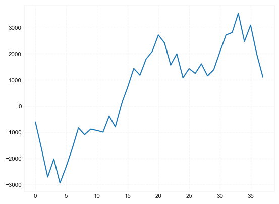
Entry 2:
- BUY when all the following criteria are met
- 30-period SMA above 9-period EMA
- 5-period RSI < 50
- 30-period VPN crosses over 30-period moving average of 30-period VPN
#entry2:
#(df['VPN']>10) & (df['VPN'].shift(1)<=10) &
df['SIGNAL'] = (df['EMA']<df['SMA']) & (df['RSI']<50)  & (df['VPN'] >= df['MA_VPN']) & (df['VPN'].shift(1) < df['MA_VPN'].shift(1))
df['B'] = df['SIGNAL']*(df["High"] + df["Low"])/2
df['SIGNAL'].value_counts()
False    5672
True       38
Name: SIGNAL, dtype: int64
trades = []
for i in range(df.shape[0]-5):
    row = df.iloc[i]
    if row['SIGNAL']>0:
        print('enter: ', i)
        row_j = df.iloc[i+1]
        item = dict(signal_date = row.name,
                    enter_date = row_j.name,
                    enter_price = row_j['High']
                   )
        for j in range(i+2, min(i+TRADE_CONFIG['HOLD_DAYS'], df.shape[0])):
            row_j = df.iloc[j]
            price_ = row_j['Low']
            pct_chg = price_/item['enter_price']
            if (pct_chg<= (1 - TRADE_CONFIG['STOP_LOSS'])) | (pct_chg >= (1 + TRADE_CONFIG['KEEP_PROFIT'])):
                break

        item['exit_date'] = row_j.name
        item['exit_price'] = price_
        item['hold_days'] = j - i
        i = j
        print('exit:', i)
        trades.append(item)
enter:  103
exit: 142
enter:  416
exit: 431
enter:  638
exit: 640
enter:  796
exit: 807
enter:  1039
exit: 1052
enter:  1055
exit: 1077
enter:  1058
exit: 1090
enter:  1161
exit: 1180
enter:  1379
exit: 1418
enter:  1387
exit: 1426
enter:  1492
exit: 1531
enter:  1721
exit: 1760
enter:  1976
exit: 1991
enter:  2041
exit: 2080
enter:  2236
exit: 2247
enter:  2309
exit: 2321
enter:  2621
exit: 2649
enter:  2766
exit: 2805
enter:  2825
exit: 2839
enter:  2931
exit: 2970
enter:  3466
exit: 3496
enter:  3671
exit: 3710
enter:  3862
exit: 3901
enter:  3886
exit: 3925
enter:  3944
exit: 3959
enter:  4037
exit: 4076
enter:  4240
exit: 4279
enter:  4260
exit: 4299
enter:  4417
exit: 4456
enter:  4434
exit: 4473
enter:  4510
exit: 4538
enter:  4767
exit: 4806
enter:  4858
exit: 4897
enter:  5088
exit: 5100
enter:  5222
exit: 5240
enter:  5479
exit: 5493
enter:  5673
exit: 5688
enter:  5699
exit: 5707
df_trades = pd.DataFrame(data = trades)
df_trades.shape
(38, 6)
df_trades['pnl'] = df_trades.apply(lambda x: cal_pnl(x), axis=1)
df_trades['pnl'].sum(), (df_trades['pnl']>0).mean()
(1103.5304500000034, 0.5526315789473685)
df_trades
| signal_date | enter_date | enter_price | exit_date | exit_price | hold_days | pnl | |
|---|---|---|---|---|---|---|---|
| 0 | 2000-05-30 | 2000-05-31 | 20.39 | 2000-07-25 | 19.21 | 39 | -613.168850 |
| 1 | 2001-08-24 | 2001-08-27 | 19.75 | 2001-09-21 | 17.79 | 15 | -1026.737250 |
| 2 | 2002-07-19 | 2002-07-22 | 13.50 | 2002-07-23 | 12.10 | 2 | -1070.965000 |
| 3 | 2003-03-06 | 2003-03-07 | 13.47 | 2003-03-21 | 14.44 | 11 | 684.758410 |
| 4 | 2004-02-23 | 2004-02-24 | 17.48 | 2004-03-11 | 15.94 | 13 | -915.874960 |
| 5 | 2004-03-16 | 2004-03-17 | 15.98 | 2004-04-16 | 17.03 | 22 | 621.293750 |
| 6 | 2004-03-19 | 2004-03-22 | 16.13 | 2004-05-05 | 17.32 | 32 | 701.664355 |
| 7 | 2004-08-17 | 2004-08-18 | 16.23 | 2004-09-14 | 17.56 | 19 | 784.288120 |
| 8 | 2005-06-28 | 2005-06-29 | 20.65 | 2005-08-23 | 20.19 | 39 | -257.621100 |
| 9 | 2005-07-11 | 2005-07-12 | 20.47 | 2005-09-02 | 20.97 | 39 | 209.037240 |
| 10 | 2005-12-07 | 2005-12-08 | 21.77 | 2006-02-03 | 21.74 | 39 | -48.743505 |
| 11 | 2006-11-03 | 2006-11-06 | 23.74 | 2007-01-03 | 23.67 | 39 | -64.450890 |
| 12 | 2007-11-09 | 2007-11-12 | 22.75 | 2007-12-03 | 24.23 | 15 | 614.764625 |
| 13 | 2008-02-14 | 2008-02-15 | 20.57 | 2008-04-11 | 19.79 | 39 | -414.069570 |
| 14 | 2008-11-20 | 2008-11-21 | 15.87 | 2008-12-08 | 17.31 | 11 | 872.206650 |
| 15 | 2009-03-10 | 2009-03-11 | 13.81 | 2009-03-26 | 14.74 | 12 | 638.325460 |
| 16 | 2010-06-04 | 2010-06-07 | 17.82 | 2010-07-15 | 19.17 | 28 | 722.360430 |
| 17 | 2010-12-30 | 2010-12-31 | 21.05 | 2011-02-25 | 20.58 | 39 | -258.245625 |
| 18 | 2011-03-25 | 2011-03-28 | 20.72 | 2011-04-14 | 22.07 | 14 | 615.745360 |
| 19 | 2011-08-25 | 2011-08-26 | 23.49 | 2011-10-20 | 24.26 | 39 | 292.308625 |
| 20 | 2013-10-11 | 2013-10-14 | 31.09 | 2013-11-22 | 33.16 | 30 | 629.540385 |
| 21 | 2014-08-06 | 2014-08-07 | 30.60 | 2014-10-01 | 29.77 | 39 | -305.494600 |
| 22 | 2015-05-11 | 2015-05-12 | 30.32 | 2015-07-07 | 27.87 | 39 | -840.963480 |
| 23 | 2015-06-15 | 2015-06-16 | 29.04 | 2015-08-10 | 30.38 | 39 | 425.995840 |
| 24 | 2015-09-04 | 2015-09-08 | 28.16 | 2015-09-28 | 25.67 | 15 | -918.938800 |
| 25 | 2016-01-20 | 2016-01-21 | 27.34 | 2016-03-16 | 28.40 | 39 | 351.973150 |
| 26 | 2016-11-07 | 2016-11-08 | 29.31 | 2017-01-04 | 28.88 | 39 | -181.611485 |
| 27 | 2016-12-06 | 2016-12-07 | 27.99 | 2017-02-02 | 29.11 | 39 | 364.866495 |
| 28 | 2017-07-24 | 2017-07-25 | 32.21 | 2017-09-18 | 30.84 | 39 | -459.647850 |
| 29 | 2017-08-16 | 2017-08-17 | 30.54 | 2017-10-11 | 31.36 | 39 | 233.186970 |
| 30 | 2017-12-04 | 2017-12-05 | 27.56 | 2018-01-16 | 29.53 | 28 | 678.221480 |
| 31 | 2018-12-12 | 2018-12-13 | 31.53 | 2019-02-08 | 33.70 | 39 | 652.907465 |
| 32 | 2019-04-25 | 2019-04-26 | 33.93 | 2019-06-20 | 34.36 | 39 | 91.506030 |
| 33 | 2020-03-24 | 2020-03-25 | 31.63 | 2020-04-09 | 34.07 | 12 | 736.057220 |
| 34 | 2020-10-02 | 2020-10-05 | 34.11 | 2020-10-28 | 30.56 | 18 | -1075.129805 |
| 35 | 2021-10-11 | 2021-10-12 | 37.48 | 2021-10-29 | 39.95 | 14 | 622.126120 |
| 36 | 2022-07-20 | 2022-07-21 | 41.82 | 2022-08-10 | 37.35 | 15 | -1103.312430 |
| 37 | 2022-08-25 | 2022-08-26 | 34.06 | 2022-09-07 | 31.16 | 8 | -884.628530 |
df_trades['pnl'].cumsum().plot()
<AxesSubplot:>