Adaptive Moving Averages

References

traders.com: TradersTips 2018-04

Definition

In "Adaptive Moving Averages" in this issue, author Vitali Apirine introduces an adaptive moving average (AMA) technique based on Perry Kaufman's KAMA (Kaufman adaptive moving average). His update to the original KAMA allows the new method to account for the location of the close relative to the high–low range. The author describes a trading system that combines the AMA and KAMA, suggesting that the combination may reduce the number of whipsaws relative to using either moving average by itself.

█ STRATEGY

if  AMA  crosses over KAMA then
    Buy TradeSize shares next bar at Market
else if  AMA  crosses under KAMA then
    Sell Short TradeSize shares next bar at Market ;
  

png

Load basic packages

import pandas as pd
import numpy as np
import os
import gc
import copy
from pathlib import Path
from datetime import datetime, timedelta, time, date
  

#this package is to download equity price data from yahoo finance
#the source code of this package can be found here: https://github.com/ranaroussi/yfinance/blob/main
import yfinance as yf
  

pd.options.display.max_rows = 100
pd.options.display.max_columns = 100

import warnings
warnings.filterwarnings("ignore")

import pytorch_lightning as pl
random_seed=1234
pl.seed_everything(random_seed)
  

Global seed set to 1234

1234

#S&P 500 (^GSPC),  Dow Jones Industrial Average (^DJI), NASDAQ Composite (^IXIC)
#Russell 2000 (^RUT), Crude Oil Nov 21 (CL=F), Gold Dec 21 (GC=F)
#Treasury Yield 10 Years (^TNX)
#CBOE Volatility Index (^VIX) Chicago Options - Chicago Options Delayed Price. Currency in USD

#benchmark_tickers = ['^GSPC', '^DJI', '^IXIC', '^RUT',  'CL=F', 'GC=F', '^TNX']

benchmark_tickers = ['^GSPC', '^VIX']
tickers = benchmark_tickers + ['GSK', 'DAL', 'PFE']
  

#https://github.com/ranaroussi/yfinance/blob/main/yfinance/base.py
#     def history(self, period="1mo", interval="1d",
#                 start=None, end=None, prepost=False, actions=True,
#                 auto_adjust=True, back_adjust=False,
#                 proxy=None, rounding=False, tz=None, timeout=None, **kwargs):

dfs = {}

for ticker in tickers:
    cur_data = yf.Ticker(ticker)
    hist = cur_data.history(period="max", start='2000-01-01')
    print(datetime.now(), ticker, hist.shape, hist.index.min(), hist.index.max())
    dfs[ticker] = hist
  

2022-09-10 18:29:09.119977 ^GSPC (5710, 7) 1999-12-31 00:00:00 2022-09-09 00:00:00
2022-09-10 18:29:09.377239 ^VIX (5710, 7) 1999-12-31 00:00:00 2022-09-09 00:00:00
2022-09-10 18:29:09.603672 GSK (5710, 7) 1999-12-31 00:00:00 2022-09-09 00:00:00
2022-09-10 18:29:09.786497 DAL (3867, 7) 2007-05-03 00:00:00 2022-09-09 00:00:00
2022-09-10 18:29:10.163955 PFE (5710, 7) 1999-12-31 00:00:00 2022-09-09 00:00:00
  

ticker = 'DAL'
dfs[ticker].tail(5)
  

	Open	High	Low	Close	Volume	Dividends	Stock Splits
Date
2022-09-02	31.440001	31.830000	30.700001	30.940001	8626500	0.0	0
2022-09-06	31.340000	31.650000	30.660000	31.190001	7630800	0.0	0
2022-09-07	31.290001	32.340000	31.270000	32.230000	9035900	0.0	0
2022-09-08	31.719999	32.490002	31.549999	32.119999	11085400	0.0	0
2022-09-09	32.430000	32.759998	32.240002	32.660000	10958900	0.0	0

TradeStation

Indicator: Adaptive Moving Average

// TASC APR 2018
// Adaptive Moving Average
// Indicator
// Vitali Apirine

inputs:
    Periods( 10 ),
    FastAvgLength( 2 ),
    SlowAvgLength( 30 ) ;

variables:
    AMA( 0 ),
    KAMA( 0 ) ;

AMA = _AMA( Periods, FastAvgLength, 
    SlowAvgLength ) ;	
KAMA = AdaptiveMovAvg( Close, Periods, 
    FastAvgLength, SlowAvgLength ) ;	

Plot1( AMA, "AMA", Cyan ) ;
Plot2( KAMA, "KAMA", Magenta ) ;

if AlertEnabled then 
begin
    if AMA crosses over KAMA then
        Alert( "AMA crossing over KAMA" ) 
    else if AMA crosses under KAMA then
        Alert( "AMA crossing under KAMA" ) ;
end ;




Strategy: Adaptive Moving Average

// TASC APR 2018
// Adaptive Moving Average
// Strategy
// Vitali Apirine

inputs:
    Periods( 10 ),
    FastAvgLength( 2 ),
    SlowAvgLength( 30 ),
    Capital( 100000 ) ;

variables:
    AMA( 0 ),
    KAMA( 0 ),
    TradeSize( 0 ) ;

AMA = _AMA( Periods, FastAvgLength, 
    SlowAvgLength ) ;	
KAMA = AdaptiveMovAvg( Close, Periods, 
    FastAvgLength, SlowAvgLength ) ;	

TradeSize = MaxList( 1, Capital / Close ) ;	

if  AMA  crosses over KAMA then
    Buy TradeSize shares next bar at Market
else if  AMA  crosses under KAMA then
    Sell Short TradeSize shares next bar at Market ;


Function: _AMA

// TASC APR 2018
// _AMA
// Function
// Vitali Apirine

inputs:
    Periods( numericsimple ),
    FastAvgLength( numericsimple ),
    SlowAvgLength( numericsimple ) ;

variables:
    PDS( Periods + 1 ),
    FastSC( 2 / ( FastAvgLength + 1 ) ),
    SlowSC( 2 / ( SlowAvgLength + 1 ) ),
    SSC( 0 ),
    CST( 0 ),
    MLTP( 0 );	

MLTP = AbsValue( ( Close - Lowest( Low, PDS ) ) 
    - ( Highest( High, PDS ) - Close )) 
    / ( Highest( High, PDS ) - Lowest( Low, PDS ) ) ;	

SSC = MLTP * ( FastSC - SlowSC ) + SlowSC ;	

CST = Square( SSC ) ;

if CurrentBar = 1 then
    _AMA = Close[1] + CST * ( Close - Close[1] )  
else
    _AMA = _AMA[1] + CST * ( Close - _AMA[1] ) ;	
  

def cal_ama(ohlc: pd.DataFrame, 
              period: int = 10, 
              fast_period: int = 2, 
              slow_period: int = 30, 
             ) -> pd.Series:
    
    """
    ADAPTIVE MOVING AVERAGE. Author: Vitali Apirine, TASC April 2018
    source: https://traders.com/documentation/feedbk_docs/2018/04/traderstips.html
    
    created on: 2022-09-10

    """
    
    ohlc = ohlc.copy()
    ohlc.columns = [c.lower() for c in ohlc.columns]
    
    highest_high = ohlc["high"].rolling(center=False, window=period).max()
    lowest_low = ohlc["low"].rolling(center=False, window=period).min()
    close = ohlc["close"]
    
    pds = period + 1
    fast_sc = 2/(fast_period + 1)
    slow_sc = 2/(slow_period + 1)
    mltp = np.abs((close - lowest_low) - (highest_high - close))/(highest_high - lowest_low)
    ssc = mltp * (fast_sc - slow_sc) + slow_sc
    cst = ssc*ssc
    
    _ama = np.zeros(len(ohlc))
    for i in range(len(ohlc)):
        if i < period:
            _ama[i] = close[i-1] + cst[i] * (close[i] - close[i-1])
        else:
            _ama[i] = _ama[i-1] + cst[i] * (close[i] - _ama[i-1])
        

    return pd.Series(_ama,index=ohlc.index, name=f"AMA")    

  

Calculate

df = dfs[ticker][['Open', 'High', 'Low', 'Close', 'Volume']]
df = df.round(2)
  

cal_ama

<function __main__.cal_ama(ohlc: pandas.core.frame.DataFrame, period: int = 10, fast_period: int = 2, slow_period: int = 30) -> pandas.core.series.Series>
  

df['AMA'] = cal_ama(df, period = 10, fast_period = 2, slow_period = 30)
  

from core.finta import TA
  

TA.KAMA
  

<function core.finta.TA.KAMA(ohlc: pandas.core.frame.DataFrame, er_period: int = 10, ema_fast: int = 2, ema_slow: int = 30, period: int = 20, column: str = 'close') -> pandas.core.series.Series>
  

df['KAMA'] = TA.KAMA(df, er_period = 10, ema_fast = 2, ema_slow=30, period=10, column='close')
  

#AMA  crosses over KAMA 
df['SIGNAL'] = ((df['AMA']>=df['KAMA']) & (df['AMA'].shift(1)<df['KAMA'].shift(1))).astype(int)
df['B'] = df['SIGNAL']*(df["High"] + df["Low"])/2
  

df['SIGNAL'].value_counts()
  

0    3754
1     113
Name: SIGNAL, dtype: int64
  

display(df.head(5))
display(df.tail(5))
  

	Open	High	Low	Close	Volume	AMA	KAMA	SIGNAL	B
Date
2007-05-03	19.32	19.50	18.25	18.40	8052800	NaN	NaN	0	0.0
2007-05-04	18.88	18.96	18.39	18.64	5437300	NaN	NaN	0	0.0
2007-05-07	18.83	18.91	17.94	18.08	2646300	NaN	NaN	0	0.0
2007-05-08	17.76	17.76	17.14	17.44	4166100	NaN	NaN	0	0.0
2007-05-09	17.54	17.94	17.44	17.58	7541100	NaN	NaN	0	0.0

	Open	High	Low	Close	Volume	AMA	KAMA	SIGNAL	B
Date
2022-09-02	31.44	31.83	30.70	30.94	8626500	31.657433	32.392120	0	0.0
2022-09-06	31.34	31.65	30.66	31.19	7630800	31.610105	32.339471	0	0.0
2022-09-07	31.29	32.34	31.27	32.23	9035900	31.616398	32.337489	0	0.0
2022-09-08	31.72	32.49	31.55	32.12	11085400	31.618872	32.328516	0	0.0
2022-09-09	32.43	32.76	32.24	32.66	10958900	31.669552	32.345109	0	0.0

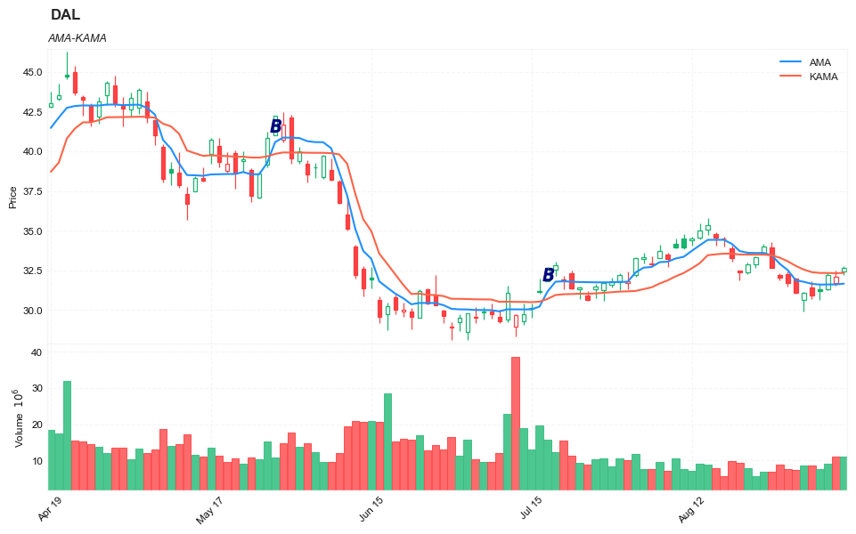
from core.visuals import *
  

start = -100
end = df.shape[0]
df_sub = df.iloc[start:end]
# df_sub = df[(df.index<='2019-04-01') & (df.index>='2019-01-24')]
names = {'main_title': f'{ticker}'}
  

lines0 = basic_lines(df_sub[['AMA', 'KAMA']], 
                     colors = [], 
                     **dict(panel=0, width=1.5, secondary_y=False))


lines2 = basic_lines(df_sub[[ 'B']],
                     colors = ['navy'], 
                     **dict(panel=0, type='scatter', marker=r'${B}$' , markersize=100, secondary_y=False))


lines_ = dict(**lines0, **lines2)

#shadows_ = basic_shadows(bands=[-0.01, 0.01], nsamples=df.iloc[start:end].shape[0], **dict(panel=1, color="lightskyblue",alpha=0.1,interpolate=True))
shadows_ = []
fig_config_ = dict(figratio=(18,10), volume=True, volume_panel=1,panel_ratios=(4,2), tight_layout=True, returnfig=True,)

ax_cfg_ = {0:dict(basic=[4, 2, ['AMA', 'KAMA']], 
                 title=dict(label = 'AMA-KAMA', fontsize=9, style='italic',  loc='left'), 
                ),
          }


names = {'main_title': f'{ticker}'}

aa_, bb_ = make_panels(main_data = df_sub[['Open', 'High', 'Low', 'Close', 'Volume']], 
                       added_plots = lines_,
                       fill_betweens = shadows_, 
                       fig_config = fig_config_, 
                       axes_config = ax_cfg_,  
                       names = names)
  

png

Simulate

TRADE_CONFIG = dict(INIT_CAPITAL = 10000 ,
                    MIN_TRADE_SIZE = 100 ,
                    MAX_TRADE_SIZE = 1000 ,
                    HOLD_DAYS = 40, #max hold days
                    STOP_LOSS = 0.085, #10% drop
                    KEEP_PROFIT = 0.065, 
                    MAX_OPEN = 1, #allow only 1 open position
                    COST = 0.0035,
                   ) 
  

df['SIGNAL'].value_counts()
  

0    3754
1     113
Name: SIGNAL, dtype: int64
  

trades = []
for i in range(df.shape[0]-5):
    row = df.iloc[i]
    if row['SIGNAL']>0:
        print('enter: ', i)
        row_j = df.iloc[i+1]
        item = dict(signal_date = row.name,
                    enter_date = row_j.name, 
                    enter_price = row_j['High']
                   )
        for j in range(i+2, min(i+TRADE_CONFIG['HOLD_DAYS'], df.shape[0])):
            row_j = df.iloc[j]
            price_ = row_j['Low']
            pct_chg = price_/item['enter_price']
            if (pct_chg<= (1 - TRADE_CONFIG['STOP_LOSS'])) | (pct_chg >= (1 + TRADE_CONFIG['KEEP_PROFIT'])):
                break
                
        item['exit_date'] = row_j.name
        item['exit_price'] = price_
        item['hold_days'] = j - i
        i = j 
        print('exit:', i)
        trades.append(item)
        
  

enter:  35
exit: 52
enter:  76
exit: 83
enter:  102
exit: 110
enter:  138
exit: 140
enter:  147
exit: 149
enter:  176
exit: 178
enter:  210
exit: 212
enter:  304
exit: 306
enter:  336
exit: 339
enter:  368
exit: 374
enter:  379
exit: 381
enter:  397
exit: 399
enter:  469
exit: 471
enter:  525
exit: 528
enter:  563
exit: 586
enter:  572
exit: 594
enter:  585
exit: 588
enter:  592
exit: 597
enter:  618
exit: 623
enter:  636
exit: 652
enter:  662
exit: 664
enter:  703
exit: 729
enter:  762
exit: 769
enter:  804
exit: 808
enter:  836
exit: 853
enter:  899
exit: 907
enter:  1006
exit: 1028
enter:  1020
exit: 1024
enter:  1041
exit: 1052
enter:  1100
exit: 1107
enter:  1120
exit: 1142
enter:  1142
exit: 1147
enter:  1156
exit: 1178
enter:  1183
exit: 1192
enter:  1194
exit: 1210
enter:  1237
exit: 1258
enter:  1249
exit: 1268
enter:  1277
exit: 1282
enter:  1294
exit: 1313
enter:  1366
exit: 1397
enter:  1391
exit: 1395
enter:  1412
exit: 1421
enter:  1443
exit: 1469
enter:  1498
exit: 1508
enter:  1535
exit: 1563
enter:  1599
exit: 1619
enter:  1680
exit: 1692
enter:  1706
exit: 1720
enter:  1735
exit: 1749
enter:  1754
exit: 1783
enter:  1834
exit: 1866
enter:  1881
exit: 1891
enter:  1942
exit: 1951
enter:  1964
exit: 1973
enter:  1981
exit: 1988
enter:  2003
exit: 2029
enter:  2021
exit: 2026
enter:  2048
exit: 2055
enter:  2061
exit: 2082
enter:  2093
exit: 2109
enter:  2121
exit: 2135
enter:  2164
exit: 2184
enter:  2192
exit: 2194
enter:  2213
exit: 2236
enter:  2233
exit: 2259
enter:  2277
exit: 2295
enter:  2312
exit: 2351
enter:  2355
exit: 2394
enter:  2366
exit: 2393
enter:  2384
exit: 2400
enter:  2409
exit: 2448
enter:  2436
exit: 2475
enter:  2517
exit: 2543
enter:  2534
exit: 2563
enter:  2609
exit: 2629
enter:  2659
exit: 2676
enter:  2693
exit: 2702
enter:  2731
exit: 2747
enter:  2761
exit: 2800
enter:  2785
exit: 2806
enter:  2810
exit: 2829
enter:  2818
exit: 2834
enter:  2867
exit: 2875
enter:  2888
exit: 2915
enter:  2958
exit: 2997
enter:  2983
exit: 3000
enter:  2997
exit: 3000
enter:  3021
exit: 3038
enter:  3043
exit: 3063
enter:  3113
exit: 3126
enter:  3126
exit: 3150
enter:  3157
exit: 3196
enter:  3165
exit: 3199
enter:  3227
exit: 3233
enter:  3233
exit: 3237
enter:  3288
exit: 3290
enter:  3352
exit: 3366
enter:  3383
exit: 3397
enter:  3405
exit: 3417
enter:  3450
exit: 3460
enter:  3465
exit: 3475
enter:  3504
exit: 3510
enter:  3515
exit: 3554
enter:  3534
exit: 3563
enter:  3606
exit: 3631
enter:  3611
exit: 3626
enter:  3624
exit: 3643
enter:  3653
exit: 3656
enter:  3668
exit: 3672
enter:  3713
exit: 3721
enter:  3745
exit: 3765
enter:  3795
exit: 3799
enter:  3829
exit: 3861
  

df_trades = pd.DataFrame(data = trades)
df_trades.shape
  

(113, 6)

def cal_pnl(trade):
    shares = int(TRADE_CONFIG['INIT_CAPITAL']/trade['enter_price'])
    if shares < TRADE_CONFIG['MIN_TRADE_SIZE']:
        shares = 0
    elif shares > TRADE_CONFIG['MAX_TRADE_SIZE']:
        shares = TRADE_CONFIG['MAX_TRADE_SIZE']
    pnl = shares*(trade['exit_price'] - trade['enter_price']) - shares*trade['enter_price']*TRADE_CONFIG['COST']
    return pnl
  

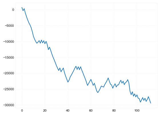
df_trades['pnl'] = df_trades.apply(lambda x: cal_pnl(x), axis=1)
  

df_trades['pnl'].sum(), (df_trades['pnl']>0).mean()
  

(-29470.04119500001, 0.4336283185840708)

df_trades

	signal_date	enter_date	enter_price	exit_date	exit_price	hold_days	pnl
0	2007-06-22	2007-06-25	17.53	2007-07-18	18.79	17	683.227650
1	2007-08-21	2007-08-22	16.57	2007-08-30	14.94	7	-1017.860985
2	2007-09-27	2007-09-28	15.95	2007-10-09	17.06	8	659.913550
3	2007-11-16	2007-11-19	17.54	2007-11-20	15.13	2	-1408.692300
4	2007-11-30	2007-12-03	17.76	2007-12-04	15.86	2	-1104.696080
...	...	...	...	...	...	...	...
108	2021-11-24	2021-11-26	36.95	2021-12-01	33.40	4	-993.417750
109	2022-01-31	2022-02-01	40.57	2022-02-10	43.31	8	639.109230
110	2022-03-17	2022-03-18	37.92	2022-04-14	41.33	20	861.924640
111	2022-05-27	2022-05-31	42.45	2022-06-03	38.06	4	-1066.565125
112	2022-07-19	2022-07-20	33.08	2022-09-01	29.94	32	-983.245560

113 rows × 7 columns

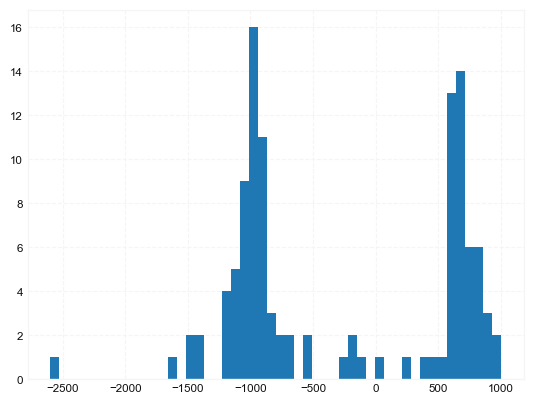
df_trades['pnl'].hist(bins=50)
  

<AxesSubplot:>

png

df_trades['pnl'].cumsum().plot()
  

<AxesSubplot:>

png