Combining Bollinger Bands With Candlesticks
References
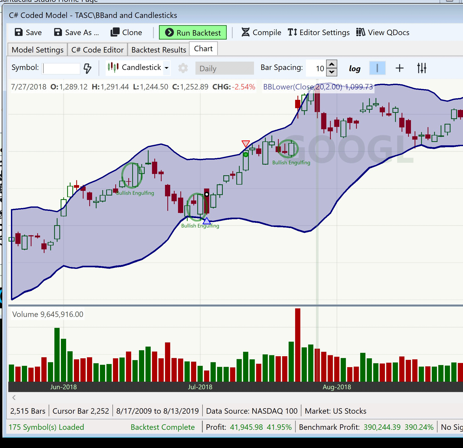
█ OVERVIEW
In "Combining Bollinger Bands With Candlesticks" in this issue, author Pawel Kosinski introduces us to a trading strategy that combines standard Bollinger Bands with the bullish engulfing candlestick pattern. Along the way we get a glimpse into the author's process for trading strategy design and testing.
The strategy uses 20-period Bollinger Bands set at 2.2 standard deviations from the center average and four times a 14-period average true range for a maximum loss stop.
Quantacula Studio's candlesticks extension can automatically flag all common candlestick patterns. We used the extension to create a model based on Pawel Kosinski's concepts described in his article in this issue. Our model buys after the price touches the lower Bollinger Band, and a Bullish Engulfing candlestick pattern has also occurred. Performing a quick backtest on the Nasdaq 100 yielded modest profits of 21.7% over a 10-year period.
We decided to tweak the entry based on a simple technique we like to use. Instead of buying the next day at market open, we buy using a limit order set to the closing price of the signal bar. Most of the time, when prices gap up, they eventually retest the previous day's close during the trading day. This technique does cause some trades to "get away from you" when they never retest, but overall the value proposition is positive. Applying this simple change doubled the net profit to 42% in our backtest.
█ STRATEGY
Buy Order tab:
Formula:
stop:= Ref(C, -1) - (4 * ATR(14));
RR:= (BBandTop(C, 20, S, 2.2)-H)/ (H-RR);
el:= C > Ref(H, -1) AND Ref( EngulfingBull(), -1) AND
Ref( Alert( L < BBandBot(C, 20, S, 2.2), 2), -1) AND RR > 1.0;
xl:= H > BBandTop(C, 20, S, 2.2);
trade:= If( PREV<=0, If(el, stop, 0),
If( L<= PREV, -1, If( xl, -2, PREV)));
trade > 0 AND Ref(trade <= 0, -1)

Sell Order tab:
Formula:
stop:= Ref(C, -1) - (4 * ATR(14));
RR:= (BBandTop(C, 20, S, 2.2)-H)/ (H-RR);
el:= C > Ref(H, -1) AND Ref( EngulfingBull(), -1) AND
Ref( Alert( L < BBandBot(C, 20, S, 2.2), 2), -1) AND RR > 1.0;
xl:= H > BBandTop(C, 20, S, 2.2);
trade:= If( PREV<=0, If(el, stop, 0),
If( L<= PREV, -1, If( xl, -2, PREV)));
trade < 0

Order Type: Stop Limit
Stop or Limit Price:
stop:= Ref(C, -1) - (4 * ATR(14));
RR:= (BBandTop(C, 20, S, 2.2)-H)/ (H-RR);
el:= C > Ref(H, -1) AND Ref( EngulfingBull(), -1) AND
Ref( Alert( L < BBandBot(C, 20, S, 2.2), 2), -1) AND RR > 1.0;
xl:= H > BBandTop(C, 20, S, 2.2);
trade:= If( PREV<=0, If(el, stop, 0),
If( L<= PREV, -1, If( xl, -2, PREV)));
If( trade = -1, Ref(trade, -1), C)
Load basic packages
import pandas as pd
import numpy as np
import os
import gc
import copy
from pathlib import Path
from datetime import datetime, timedelta, time, date
#this package is to download equity price data from yahoo finance
#the source code of this package can be found here: https://github.com/ranaroussi/yfinance/blob/main
import yfinance as yf
pd.options.display.max_rows = 100
pd.options.display.max_columns = 100

import warnings
warnings.filterwarnings("ignore")

import pytorch_lightning as pl
random_seed=1234
pl.seed_everything(random_seed)
Global seed set to 1234


1234
Download data
##### Download data#S&P 500 (^GSPC),  Dow Jones Industrial Average (^DJI), NASDAQ Composite (^IXIC)
#Russell 2000 (^RUT), Crude Oil Nov 21 (CL=F), Gold Dec 21 (GC=F)
#Treasury Yield 10 Years (^TNX)
#CBOE Volatility Index (^VIX) Chicago Options - Chicago Options Delayed Price. Currency in USD

#benchmark_tickers = ['^GSPC', '^DJI', '^IXIC', '^RUT',  'CL=F', 'GC=F', '^TNX']

benchmark_tickers = ['^GSPC', '^VIX']
tickers = benchmark_tickers + ['GSK', 'BST', 'PFE','DAL']
#https://github.com/ranaroussi/yfinance/blob/main/yfinance/base.py
#     def history(self, period="1mo", interval="1d",
#                 start=None, end=None, prepost=False, actions=True,
#                 auto_adjust=True, back_adjust=False,
#                 proxy=None, rounding=False, tz=None, timeout=None, **kwargs):

dfs = {}

for ticker in tickers:
    cur_data = yf.Ticker(ticker)
    hist = cur_data.history(period="max", start='2000-01-01')
    print(datetime.now(), ticker, hist.shape, hist.index.min(), hist.index.max())
    dfs[ticker] = hist
2022-09-10 01:06:11.715775 ^GSPC (5710, 7) 1999-12-31 00:00:00 2022-09-09 00:00:00
2022-09-10 01:06:12.011806 ^VIX (5710, 7) 1999-12-31 00:00:00 2022-09-09 00:00:00
2022-09-10 01:06:12.412567 GSK (5710, 7) 1999-12-31 00:00:00 2022-09-09 00:00:00
2022-09-10 01:06:12.663710 BST (1980, 7) 2014-10-29 00:00:00 2022-09-09 00:00:00
2022-09-10 01:06:13.052159 PFE (5710, 7) 1999-12-31 00:00:00 2022-09-09 00:00:00
2022-09-10 01:06:13.314652 DAL (3867, 7) 2007-05-03 00:00:00 2022-09-09 00:00:00
ticker = 'DAL'
dfs[ticker].tail(5)
| Open | High | Low | Close | Volume | Dividends | Stock Splits | |
|---|---|---|---|---|---|---|---|
| Date | |||||||
| 2022-09-02 | 31.440001 | 31.830000 | 30.700001 | 30.940001 | 8626500 | 0.0 | 0 |
| 2022-09-06 | 31.340000 | 31.650000 | 30.660000 | 31.190001 | 7630800 | 0.0 | 0 |
| 2022-09-07 | 31.290001 | 32.340000 | 31.270000 | 32.230000 | 9035900 | 0.0 | 0 |
| 2022-09-08 | 31.719999 | 32.490002 | 31.549999 | 32.119999 | 11074800 | 0.0 | 0 |
| 2022-09-09 | 32.430000 | 32.759998 | 32.240002 | 32.435001 | 4745097 | 0.0 | 0 |
Calculate the technical indicators and Find signals
def bull_engulfing(c: pd.Series, o: pd.Series)-> pd.Series:
    """
    c: pd.Series. close price
    o: pd.Series. open price

    BULL ENGULFING: meet all of the following
        current OPEN > current CLOSE
        pre CLOSE > pre OPEN
        current CLOSE > pre OPEN
        current OPEN > pre CLOSE
    """
    be = (c>o) & (c.shift(1)<o.shift(1)) & (c>o.shift(1)) & (o<c.shift(1))
    return pd.Series(be, name='BULL_ENGULF')


def bbands_trigger(c:pd.Series, l:pd.Series, bb_lower:pd.Series) -> pd.Series:
    """
    c: pd.Series. close price
    l: pd.Series. low price
    bb_lower: lower band of Bollinger bands

    Bollinger Bands Trigger: meet all of the following
        pre CLOSE < pre BBANDS lower band
        current CLOSE > current BBANDS lower band
        current LOW < current BBANDS lower band
    """
    bt = (c.shift(1)<bb_lower.shift(1)) & (c > bb_lower) & (l < bb_lower)

    return pd.Series(bt, name='BBANDS_TRIGGER')
from core.finta import TA
df = dfs[ticker][['Open', 'High', 'Low', 'Close', 'Volume']]
df = df.round(2)
TA.BBANDS
<function core.finta.TA.BBANDS(ohlc: pandas.core.frame.DataFrame, period: int = 20, MA: pandas.core.series.Series = None, column: str = 'close', std_multiplier: float = 2) -> pandas.core.frame.DataFrame>
df_ta = TA.BBANDS(df, period = 20, std_multiplier=2.2, column="close")
df = df.merge(df_ta, left_index = True, right_index = True, how='inner' )


del df_ta
gc.collect()
15467
df['BULL_ENGULF'] = bull_engulfing(df["Close"], df["Open"])
df['BBANDS_TRIGGER'] = bbands_trigger(df["Close"], df["Low"], df["BB_LOWER"])
df['SIGNAL'] = (df['BULL_ENGULF'] & df['BBANDS_TRIGGER']).astype(int)
df['B'] = df['SIGNAL']*(df["High"] + df["Low"])/2
display(df.head(5))
display(df.tail(5))
| Open | High | Low | Close | Volume | BB_UPPER | BB_MIDDLE | BB_LOWER | BBWIDTH | PERCENT_B | BULL_ENGULF | BBANDS_TRIGGER | SIGNAL | B | |
|---|---|---|---|---|---|---|---|---|---|---|---|---|---|---|
| Date | ||||||||||||||
| 2007-05-03 | 19.32 | 19.50 | 18.25 | 18.40 | 8052800 | NaN | NaN | NaN | NaN | NaN | False | False | 0 | 0.0 |
| 2007-05-04 | 18.88 | 18.96 | 18.39 | 18.64 | 5437300 | NaN | NaN | NaN | NaN | NaN | False | False | 0 | 0.0 |
| 2007-05-07 | 18.83 | 18.91 | 17.94 | 18.08 | 2646300 | NaN | NaN | NaN | NaN | NaN | False | False | 0 | 0.0 |
| 2007-05-08 | 17.76 | 17.76 | 17.14 | 17.44 | 4166100 | NaN | NaN | NaN | NaN | NaN | False | False | 0 | 0.0 |
| 2007-05-09 | 17.54 | 17.94 | 17.44 | 17.58 | 7541100 | NaN | NaN | NaN | NaN | NaN | False | False | 0 | 0.0 |
| Open | High | Low | Close | Volume | BB_UPPER | BB_MIDDLE | BB_LOWER | BBWIDTH | PERCENT_B | BULL_ENGULF | BBANDS_TRIGGER | SIGNAL | B | |
|---|---|---|---|---|---|---|---|---|---|---|---|---|---|---|
| Date | ||||||||||||||
| 2022-09-02 | 31.44 | 31.83 | 30.70 | 30.94 | 8626500 | 36.133696 | 33.2025 | 30.271304 | 0.176565 | 0.114065 | False | False | 0 | 0.0 |
| 2022-09-06 | 31.34 | 31.65 | 30.66 | 31.19 | 7630800 | 36.150830 | 33.0745 | 29.998170 | 0.186024 | 0.193710 | False | False | 0 | 0.0 |
| 2022-09-07 | 31.29 | 32.34 | 31.27 | 32.23 | 9035900 | 36.128493 | 33.0255 | 29.922507 | 0.187915 | 0.371817 | False | False | 0 | 0.0 |
| 2022-09-08 | 31.72 | 32.49 | 31.55 | 32.12 | 11074800 | 36.031337 | 32.9350 | 29.838663 | 0.188027 | 0.368393 | False | False | 0 | 0.0 |
| 2022-09-09 | 32.43 | 32.76 | 32.24 | 32.44 | 4745097 | 35.917212 | 32.8590 | 29.800788 | 0.186141 | 0.431496 | False | False | 0 | 0.0 |
df['SIGNAL'].value_counts()
0    3864
1       3
Name: SIGNAL, dtype: int64
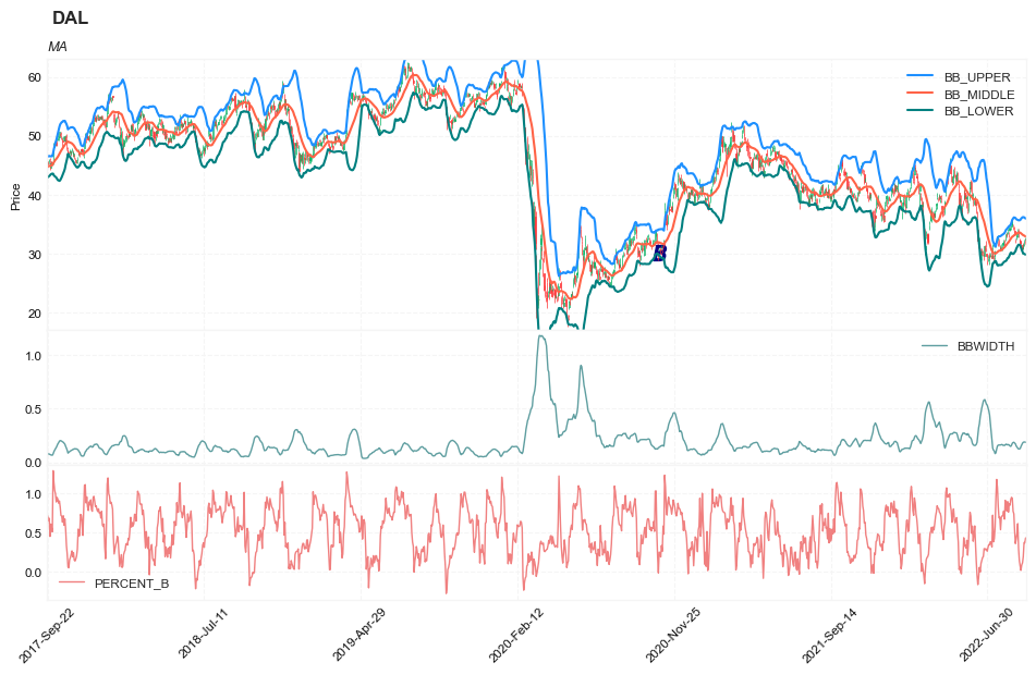
Visual
from core.visuals import *
start = -1250
end = df.shape[0]
df_sub = df.iloc[start:end]
# df_sub = df[(df.index<='2019-04-01') & (df.index>='2019-01-24')]
names = {'main_title': f'{ticker}'}
lines0 = basic_lines(df_sub[['BB_UPPER', 'BB_MIDDLE', 'BB_LOWER']],
                     colors = [],
                     **dict(panel=0, width=1.5, secondary_y=False))

lines1 = basic_lines(df_sub[['BBWIDTH']],
                     colors = ['cadetblue'],
                     **dict(panel=1, width=1))
lines3 = basic_lines(df_sub[['PERCENT_B']],
                     colors = ['lightcoral'],
                     **dict(panel=2, width=1))

lines2 = basic_lines(df_sub[[ 'B']],
                     colors = ['navy'],
                     **dict(panel=0, type='scatter', marker=r'${B}$' , markersize=100, secondary_y=False))


lines_ = dict(**lines0, **lines1)
lines_.update(lines2)
lines_.update(lines3)

#shadows_ = basic_shadows(bands=[-0.01, 0.01], nsamples=df.iloc[start:end].shape[0], **dict(panel=1, color="lightskyblue",alpha=0.1,interpolate=True))
shadows_ = []
fig_config_ = dict(figratio=(18,10), volume=False, volume_panel=2,panel_ratios=(4,2, 2), tight_layout=True, returnfig=True,)

ax_cfg_ = {0:dict(basic=[5, 2, ['BB_UPPER', 'BB_MIDDLE', 'BB_LOWER']],
                 title=dict(label = 'MA', fontsize=9, style='italic',  loc='left'),
                ),
           2:dict(basic=[1, 0, ['BBWIDTH']]
                ),
           4:dict(basic=[1, 0, ['PERCENT_B']]
                ),
          }


names = {'main_title': f'{ticker}'}

aa_, bb_ = make_panels(main_data = df_sub[['Open', 'High', 'Low', 'Close', 'Volume']],
                       added_plots = lines_,
                       fill_betweens = shadows_,
                       fig_config = fig_config_,
                       axes_config = ax_cfg_,
                       names = names)
Simulate
TRADE_CONFIG = dict(INIT_CAPITAL = 10000 ,
                    MIN_TRADE_SIZE = 100 ,
                    MAX_TRADE_SIZE = 1000 ,
                    HOLD_DAYS = 40, #max hold days
                    STOP_LOSS = 0.085, #10% drop
                    KEEP_PROFIT = 0.065,
                    MAX_OPEN = 1, #allow only 1 open position
                    COST = 0.0035,
                   )
df['SIGNAL'].value_counts()
0    3864
1       3
Name: SIGNAL, dtype: int64
trades = []
for i in range(df.shape[0]-5):
    row = df.iloc[i]
    if row['SIGNAL']>0:
        print('enter: ', i)
        row_j = df.iloc[i+1]
        item = dict(signal_date = row.name,
                    enter_date = row_j.name,
                    enter_price = row_j['High']
                   )
        for j in range(i+2, min(i+TRADE_CONFIG['HOLD_DAYS'], df.shape[0])):
            row_j = df.iloc[j]
            price_ = row_j['Low']
            pct_chg = price_/item['enter_price']
            if (pct_chg<= (1 - TRADE_CONFIG['STOP_LOSS'])) | (pct_chg >= (1 + TRADE_CONFIG['KEEP_PROFIT'])):
                break

        item['exit_date'] = row_j.name
        item['exit_price'] = price_
        item['hold_days'] = j - i
        i = j
        print('exit:', i)
        trades.append(item)
enter:  960
exit: 965
enter:  2208
exit: 2216
enter:  3398
exit: 3405
df_trades = pd.DataFrame(data = trades)
df_trades.shape
(3, 6)
def cal_pnl(trade):
    shares = int(TRADE_CONFIG['INIT_CAPITAL']/trade['enter_price'])
    if shares < TRADE_CONFIG['MIN_TRADE_SIZE']:
        shares = 0
    elif shares > TRADE_CONFIG['MAX_TRADE_SIZE']:
        shares = TRADE_CONFIG['MAX_TRADE_SIZE']
    pnl = shares*(trade['exit_price'] - trade['enter_price']) - shares*trade['enter_price']*TRADE_CONFIG['COST']
    return pnl
df_trades['pnl'] = df_trades.apply(lambda x: cal_pnl(x), axis=1)
df_trades
| signal_date | enter_date | enter_price | exit_date | exit_price | hold_days | pnl | |
|---|---|---|---|---|---|---|---|
| 0 | 2011-02-23 | 2011-02-24 | 10.05 | 2011-03-02 | 8.99 | 5 | -1089.699125 |
| 1 | 2016-02-09 | 2016-02-10 | 39.79 | 2016-02-22 | 42.59 | 8 | 667.844485 |
| 2 | 2020-10-29 | 2020-10-30 | 30.99 | 2020-11-09 | 34.68 | 7 | 1153.254270 |